Evaluating the Structural Model in SmartPLS 4: Collinearity, R² and f²
Check inner VIF, read R² and adjusted R², compute the f² effect size by hand and report weak to moderate explanatory power honestly


Key takeaways
A PLS-SEM structural model is evaluated in five steps: collinearity, path significance, R², f² and predictive power; this post covers collinearity, R² and f².
Collinearity between latent variables is read from Inner model VIF, not Outer model VIF; on the Marketplace X model the highest is 1.681, below 3.
The model explains 25.1% of perceived value, 39.9% of satisfaction and 31.8% of repurchase intention: weak to moderate, and it should be reported that way.
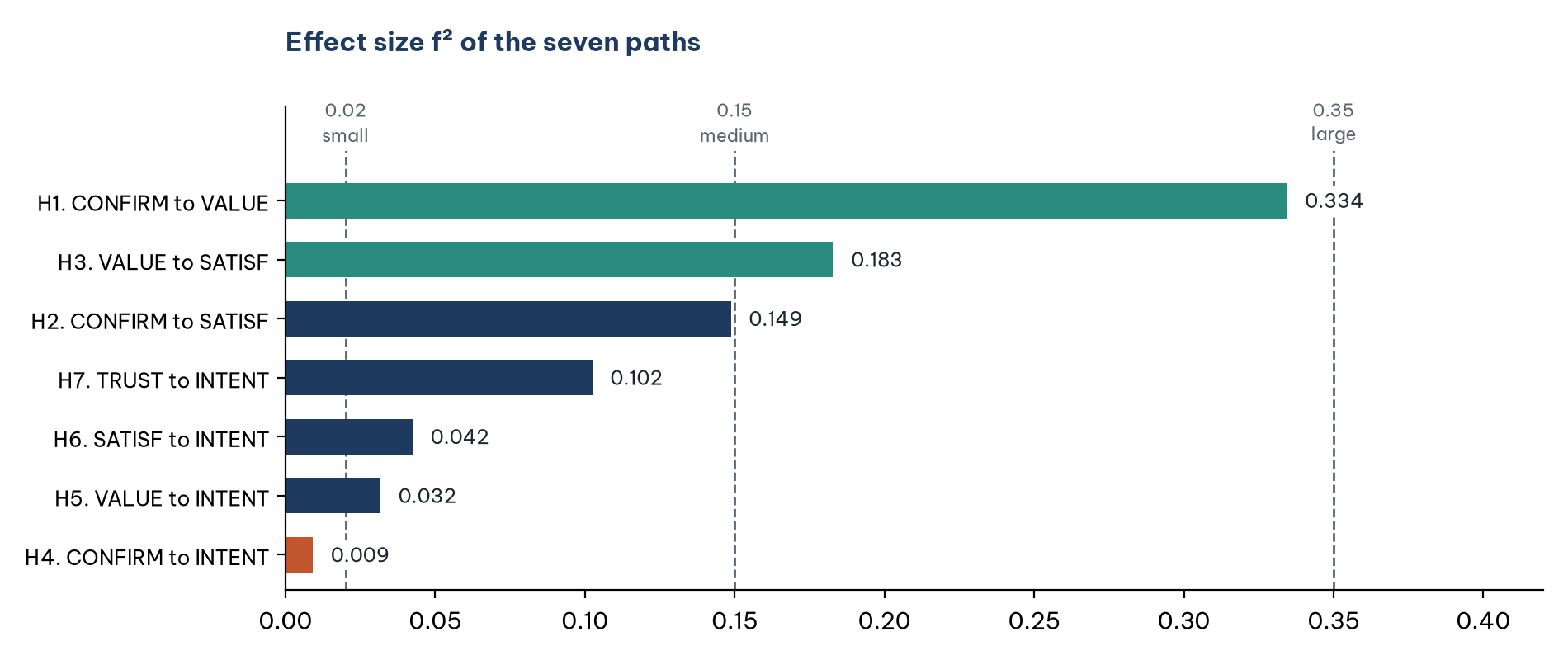
f² is the unique contribution of one predictor; trust contributes most to repurchase intention (0.102), while confirmation has almost no direct effect (0.009).
PLS-SEM gives lower R² than CB-SEM on the same data (0.318 versus 0.444 for intention), so check the method before comparing with earlier studies.
Posts 34 and 35 showed that the measurement scales of the Marketplace X model meet the requirements. From this post on, the series turns to the structural model: the relationships between the five constructs and hypotheses H1 to H7. Hair et al. (2019) recommend evaluating the structural model in five steps:
Collinearity between the latent variables (this post).
Significance and size of the path coefficients (Post 39, with bootstrapping).
Explanatory power: R² (this post).
Effect size of each predictor: f² (this post).
Predictive power: Q² and PLSpredict (Post 38).
The posts in this series follow the editorial schedule; in a thesis, present the results in the order of the five steps above.
Sample data and scripts. The data file and scripts for this post are in the research-data-analysis repository on GitHub (folder
data/andscripts/). Download the whole repository with Code > Download ZIP.
About the figures and numbers. The figures are real screenshots of the SmartPLS 4.1.2.1 report (Ringle et al., 2026; 30-day trial) for the model
marketplace-x-modelfrom Post 33, running the PLS-SEM algorithm again with casewise deletion on 254 respondents. Every number was checked in R with the scriptstructural_model.R(in the repository'sscripts/folder) and matches SmartPLS to the third decimal place. SmartPLS lists constructs and paths in alphabetical order (CONFIRM, INTENT, SATISF, TRUST, VALUE).
1. Step 1: Collinearity between the latent variables
The path coefficients of an endogenous construct are estimated like a multiple regression on the latent variables that predict it. If these predictors are too highly correlated with each other, the coefficients become biased and unstable, just as with multicollinearity in the regression of Post 15.
Step 1. In the report of the PLS-SEM algorithm, open Quality criteria > Collinearity statistics (VIF) > Inner model - List (Figure 1). The item Outer model - List in the same group gives the VIF of the indicators, which is used for formative measurement (Post 36).
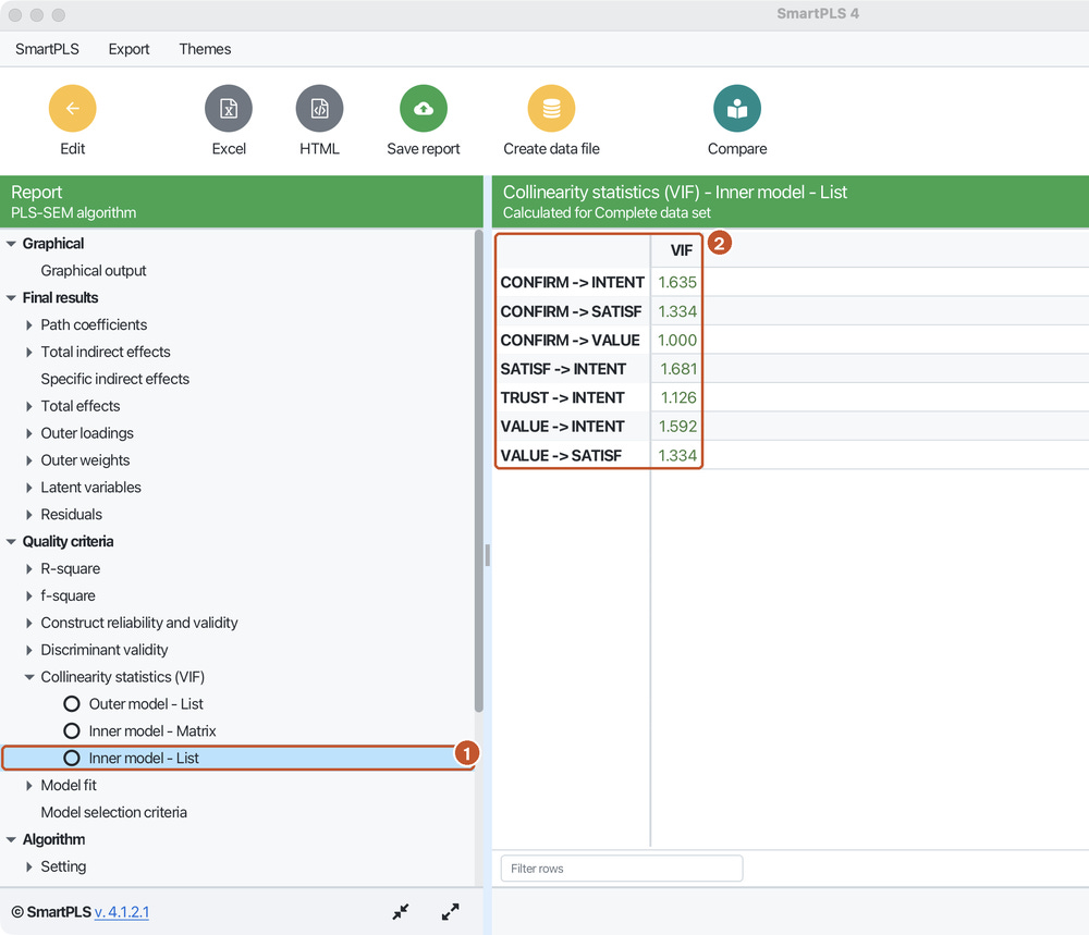
Threshold (Hair et al., 2019): a VIF of 5 or more indicates a critical problem; ideally the VIF is below 3.
Result: the highest VIF is 1.681, below 3: there is no collinearity. VALUE has only one predictor, so its VIF equals 1. For SATISF, the two predictors have the same VIF, because the VIF of each one is computed from its correlation with the other.
2. Step 3: Explanatory power (R²)
R² is the share of the variance of an endogenous construct that its predictors explain. Adjusted R² removes the part of the increase that comes only from the number of predictors; use it when comparing models with different numbers of predictors:
Adjusted R² = 1 - (1 - R²) x (n - 1) / (n - k - 1), where n is the sample size and k the number of predictors.
Step 2. Open Quality criteria > R-square > Overview (Figure 2).
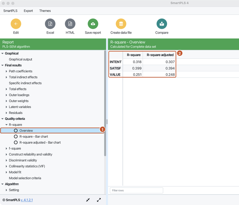
Rules of thumb (Hair et al., 2019; Hair et al., 2022): an R² of 0.75 is substantial, 0.50 moderate and 0.25 weak. These thresholds depend on the field: in consumer behavior research, lower R² values can still be acceptable, because behavior is influenced by many factors outside the model.
Hand calculation of the adjusted R² of INTENT (n = 254, k = 4): 1 - (1 - 0.318) x 253 / 249 = 1 - 0.682 x 1.016 = 0.307.
Result: the four constructs of the model explain 31.8% of the variance of repurchase intention, and two constructs explain 39.9% of the variance of satisfaction. By the thresholds of Hair et al., explanatory power is between weak and moderate. This is an honest result of the data and should be reported as such, not described as "good explanatory power".
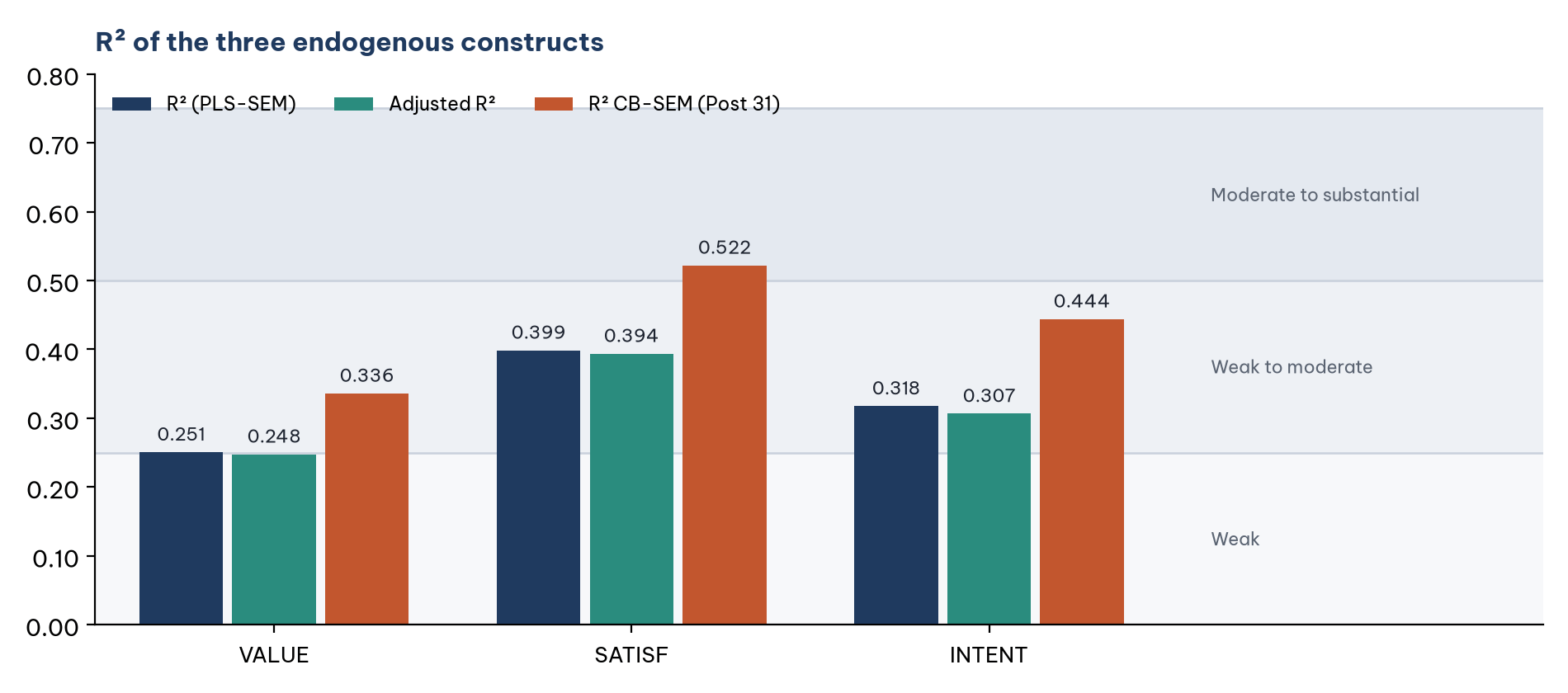
The PLS-SEM R² is lower than the CB-SEM R² for all three constructs (for example, INTENT: 0.318 versus 0.444; Post 31). This is a known bias of PLS-SEM when the constructs are common factors: the composites contain measurement error, which dilutes the relationships between constructs. When you compare R² values with earlier studies, check which method those studies used.
3. Step 4: Effect size (f²)
f² shows how much the R² of an endogenous construct drops when one predictor is removed from the model, that is, the unique contribution of that predictor:
f² = (R² included - R² excluded) / (1 - R² included)
Thresholds (Cohen, 1988): 0.02 is a small effect, 0.15 medium and 0.35 large. Values below 0.02 mean no effect.
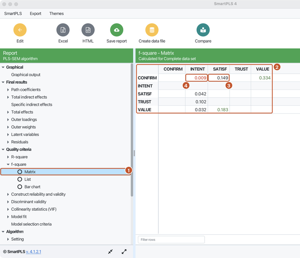
Step 3. Open Quality criteria > f-square > Matrix (Figure 4). Read it with predictors in the rows and endogenous constructs in the columns.
Hand calculation of f² for TRUST to INTENT
Take the R² of INTENT with all four predictors: 0.31755.
Run the model again without TRUST; the R² of INTENT drops to 0.24765 (script
structural_model.R).Compute f² = (0.31755 - 0.24765) / (1 - 0.31755) = 0.06990 / 0.68245 = 0.102, the same as SmartPLS.
For an endogenous construct with only one predictor (VALUE), removing that predictor makes R² equal to 0, so f² = R² / (1 - R²) = 0.251 / 0.749 = 0.334.
Reading the results:
Expectation confirmation has the largest effect, on perceived value (f² = 0.334), in line with expectation-confirmation theory.
Perceived value has a medium effect on satisfaction (0.183); the effect of confirmation on satisfaction (0.149) is just below the medium threshold. The correct report is "small, just below medium", not rounded up to "medium".
For repurchase intention, trust makes the largest unique contribution (0.102), although all four effects are small.
Confirmation has almost no direct effect on intention (f² = 0.009). This agrees with Post 31: H4 was not statistically significant (p = 0.086). The effect of confirmation on intention, if any, runs through perceived value and satisfaction; Post 40 tests this indirect effect.
4. Reporting the results
There is no collinearity between the latent variables: VIF values range from 1.000 to 1.681, below 3 (Hair et al., 2019). The model explains 25.1% of the variance of perceived value, 39.9% of satisfaction and 31.8% of repurchase intention (adjusted R² of 0.248, 0.394 and 0.307 respectively), so explanatory power is weak to moderate. In terms of effect size (Cohen, 1988), expectation confirmation has a medium effect, close to large, on perceived value (f² = 0.334); perceived value has a medium effect on satisfaction (f² = 0.183); the effects on repurchase intention are all small, with trust the largest (f² = 0.102). The direct effect of expectation confirmation on repurchase intention is negligible (f² = 0.009).
The table in a thesis should combine, for each hypothesis: the path coefficient, t, p, the confidence interval (Post 39), f² and VIF; together with the R² and adjusted R² of each endogenous construct.
Four common mistakes
Reading the VIF of the indicators (Outer model) to judge collinearity in the structural model. Read the Inner model instead.
Reading the f² matrix the wrong way round: rows are predictors, columns are endogenous constructs.
Concluding "the model is good" only because R² is statistically significant. An R² of 0.318 means that almost 70% of the variance of repurchase intention is still unexplained; mention this in the limitations and directions for future research.
Rounding effect sizes (0.149 reported as "medium"). Report against the exact thresholds; when a value is close to a threshold, say so.
Frequently asked questions
How high does R² need to be for a thesis?
There is no common threshold for every field. Compare with studies on the same topic that used the same method. The PLS-SEM R² is usually lower than the CB-SEM R² on the same data (Figure 3).
Does f² need a significance test?
f² is a measure of size; it does not replace the significance test of the path coefficient (Post 39). Report both: whether the coefficient is significant and, if it is, how large the effect is.
Should I report R² or adjusted R²?
Report both. Adjusted R² is useful when you compare models with different numbers of predictors, for example a model with and without a moderator (Post 41).
References
Cohen, J. (1988). Statistical power analysis for the behavioral sciences (2nd ed.). Lawrence Erlbaum Associates.
Hair, J. F., Hult, G. T. M., Ringle, C. M., & Sarstedt, M. (2022). A primer on partial least squares structural equation modeling (PLS-SEM) (3rd ed.). SAGE Publications.
Hair, J. F., Risher, J. J., Sarstedt, M., & Ringle, C. M. (2019). When to use and how to report the results of PLS-SEM. European Business Review, 31(1), 2–24. https://doi.org/10.1108/EBR-11-2018-0203
Ringle, C. M., Wende, S., & Becker, J.-M. (2026). SmartPLS 4 (Version 4.1.2.1) [Computer software]. SmartPLS GmbH. https://www.smartpls.com
Discussion about this post