Moderation Analysis in SmartPLS 4: Interaction, f² and Simple Slopes
Draw a moderating effect, read the interaction coefficient, f² and simple slope plot, test it with bootstrapping and report a non-significant result


Key takeaways
A moderator changes the strength of a path; in SmartPLS you draw it by connecting the moderator to the middle of that arrow.
SmartPLS 4 uses the two-stage approach: the interaction term is the product of the latent variable scores from the main-effects model.
With an interaction term in the model, a main-effect coefficient is the effect when the moderator is at its mean, not a general effect.
Trust does not moderate the effect of satisfaction on repurchase intention: coefficient −0.020 (p = 0.670) and f² = 0.001, with almost parallel simple slopes.
A non-significant moderation result should still be reported in full, with the coefficient, p, confidence interval and f².
Post 40 showed through what expectation confirmation affects repurchase intention (mediation). This post asks a different question: does the effect of one construct become stronger or weaker depending on the level of a third construct? That third construct is a moderator.
Post 29 tested a moderation hypothesis with CB-SEM: Does trust moderate the effect of satisfaction on repurchase intention? The reasoning: customers who trust Marketplace X may buy again even when they are not very satisfied, so the effect of satisfaction should be weaker when trust is high. This post tests the same hypothesis again with SmartPLS 4.
Sample data and scripts. The data file and scripts for this post are in the research-data-analysis repository on GitHub (folder
data/andscripts/). Download the whole repository with Code > Download ZIP.
About the figures and numbers. The figures are real screenshots of SmartPLS 4.1.2.1 (Ringle et al., 2026; 30-day trial) for the model
moderation-model, a copy ofmarketplace-x-model(Post 33), with casewise deletion on 254 respondents. Figure 3 (the PLS-SEM algorithm dialog) comes from an earlier capture with the same SmartPLS version; the dialog shows no project or model names. According to the SmartPLS license comparison page, the Student license does not include moderation analysis. The numbers in this post come from the SmartPLS report. Section 6 checks them in R (scriptmoderation.Rin the repository'sscripts/folder, package cSEM) and against CB-SEM in AMOS and JASP (Post 29). SmartPLS lists constructs and paths in alphabetical order (CONFIRM, INTENT, SATISF, TRUST, VALUE, TRUST x SATISF).
1. Moderator and mediator
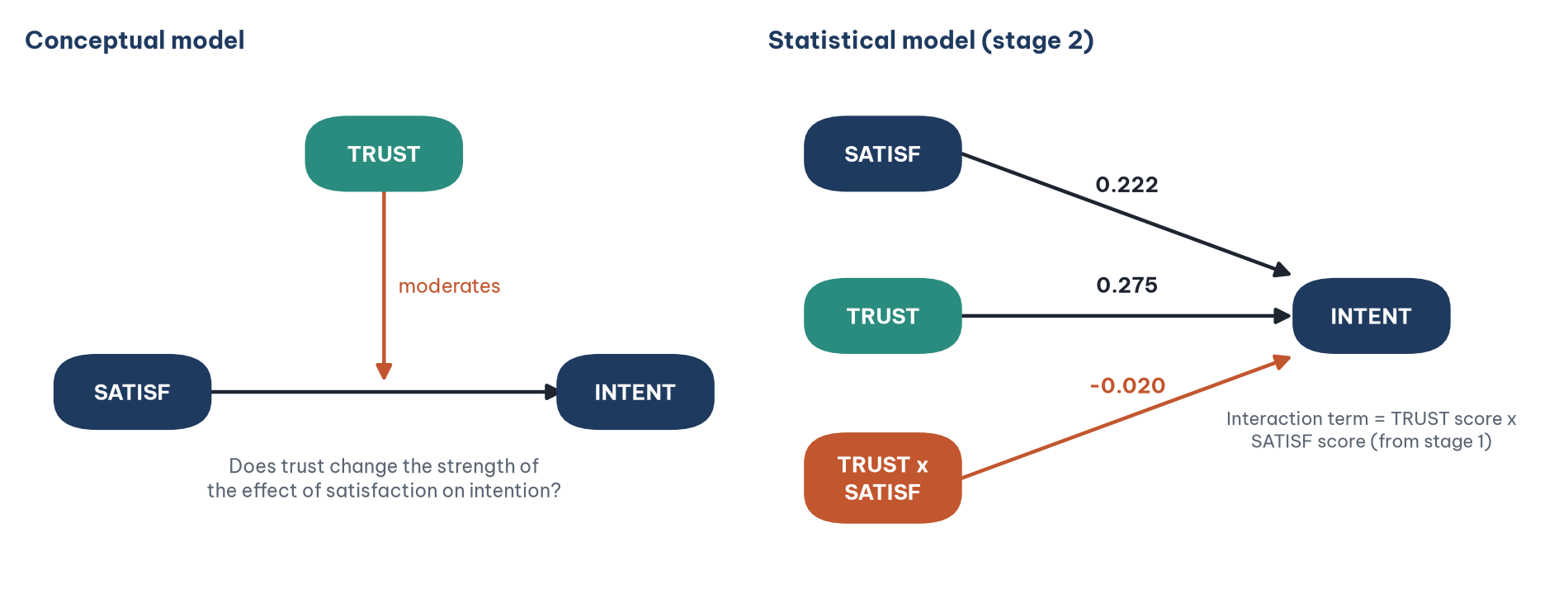
In the Marketplace X model, TRUST has a direct effect on INTENT (H7) and is also hypothesized to moderate the path from SATISF to INTENT (Figure 1).
2. How does SmartPLS estimate a moderating effect?
SmartPLS 4 uses the two-stage approach (Becker et al., 2018; Hair et al., 2022):
Stage 1. Estimate the main-effects model (without the interaction term) and obtain the latent variable scores of SATISF and TRUST.
Stage 2. Create the interaction term as the product of these two scores, use it as a single-item construct and estimate the model with the interaction term.
Two points to know:
The path from the moderator to the dependent construct. SmartPLS adds the path from the moderator to the dependent construct automatically during the calculation, because the interaction test is only correct when the model also contains the main effect of the moderator. In the Marketplace X model, the path TRUST to INTENT (H7) is already there.
The scale of the interaction term. With Type of results set to Standardized, the latent variable scores that are multiplied are standardized. Their product is kept as it is; it is not standardized again.
3. Adding the moderating effect to the model
Step 1. Create a copy of marketplace-x-model in the workspace: select the model in the Workspace pane and choose Files > Duplicate. Rename the copy moderation-model and open it. Keep the original model unchanged so that the earlier posts can still be reproduced.
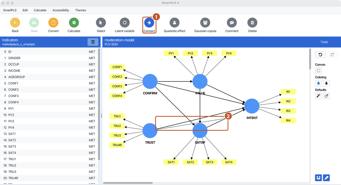
Step 2. Click the Connect button on the toolbar. Click TRUST, drag to the middle of the arrow from SATISF to INTENT and release the mouse button (Figure 2). SmartPLS draws a dashed line from TRUST that touches that arrow; there is no separate node for the interaction term on the canvas.
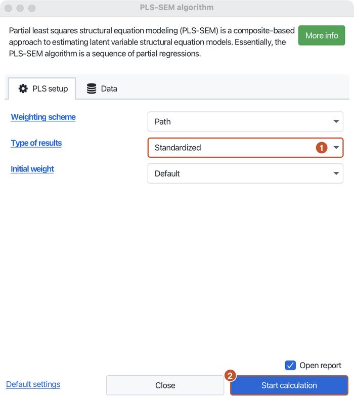
Step 3. Click Save. Choose Calculate > PLS-SEM algorithm, check that Type of results is Standardized and that the Data tab is set to Casewise deletion, then click Start calculation (Figure 3).
4. Reading the results of the PLS-SEM algorithm
The interaction coefficient
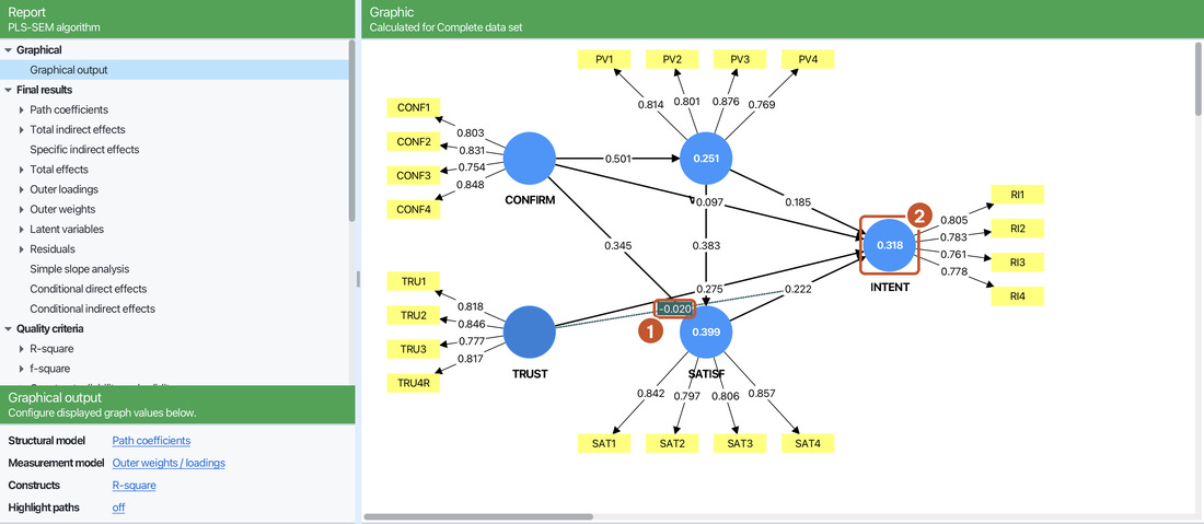
The results graph has an extra path from TRUST x SATISF to INTENT, shown as a label on the dashed line (Figure 4).
Reading the coefficients:
The interaction coefficient of −0.020 is negative, in the hypothesized direction (the higher the trust, the weaker the effect of satisfaction), but it is very small.
With the interaction term in the model, the coefficient of SATISF (0.222) is the effect of satisfaction when trust is at its mean, no longer a "general effect" as in Post 37. Likewise, 0.275 is the effect of trust when satisfaction is at its mean.
R² does not change (0.318, rounded to three decimals): the interaction term explains almost no additional variance of INTENT.
Effect size f²
Step 4. Open Quality criteria > f-square > Matrix (Figure 5).
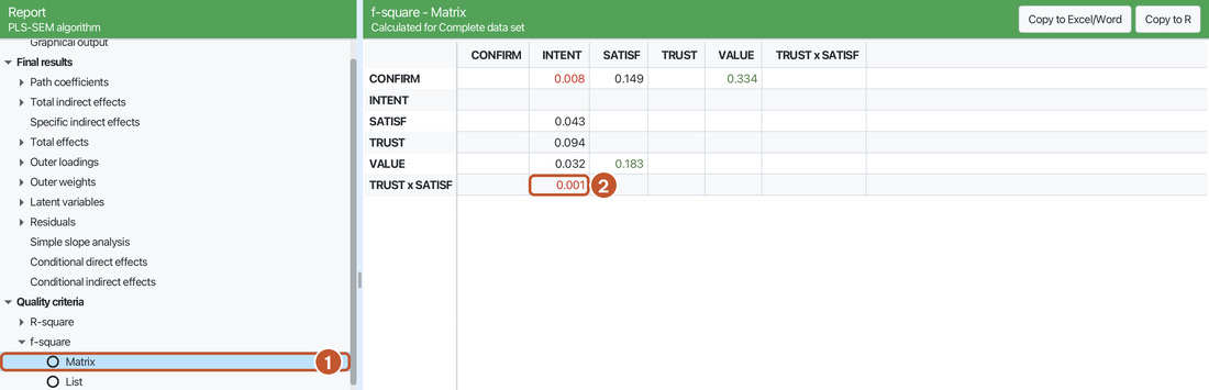
The f² of the interaction term is 0.001. For moderating effects, Cohen's threshold of 0.02 (Cohen, 1988) is too strict: in a 30-year review, Aguinis et al. (2005) found that the average f² of moderating effects (with categorical moderators) in published studies was only about 0.009. Even against this benchmark, 0.001 is very small.
Simple slopes
Step 5. Open Final results > Simple slope analysis (Figure 6).
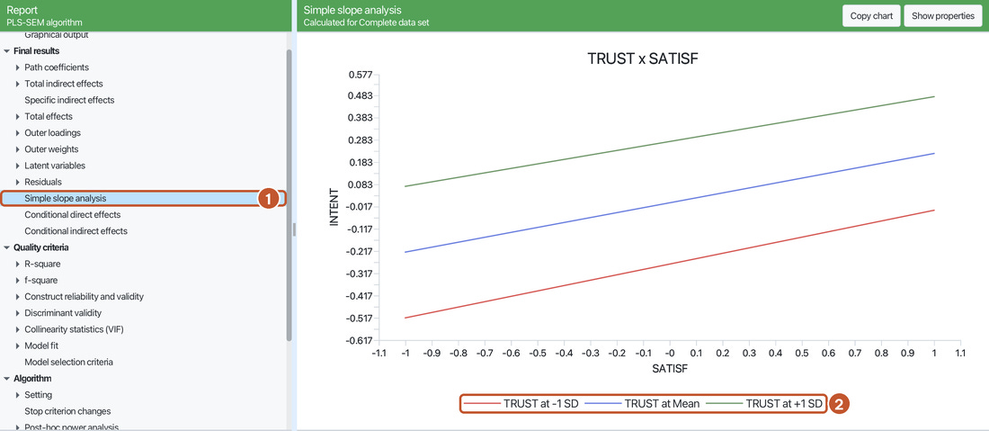
Each line shows the relationship between SATISF (horizontal axis) and INTENT (vertical axis) at one level of TRUST. Reading the plot:
The three lines are almost parallel. The slopes, computed by hand from the SmartPLS coefficients as 0.222 - 0.020 x (level of TRUST), are 0.242 when trust is low, 0.222 when it is at the mean and 0.202 when it is high. The slope decreases very little.
The distance between the lines is the main effect of TRUST (0.275): at the same level of satisfaction, respondents with high trust have a higher repurchase intention.
If there were a substantial moderating effect, the lines would not be parallel: for example, the line for high trust would be clearly flatter than the line for low trust.
5. Testing significance with bootstrapping
Step 6. Click Edit to return to the model, choose Calculate > Bootstrapping with the settings of Post 39 (5000 subsamples, Percentile bootstrap, Two-tailed, Fixed seed), then click Start calculation.
Step 7. Open Final results > Path coefficients > Mean, STDEV, T values, p values (Figure 7).

Step 8. Open Path coefficients > Confidence intervals (Figure 8).

Conclusion: the interaction coefficient is not significant (t = 0.427, p = 0.670), and the confidence interval includes 0. Trust does not moderate the effect of satisfaction on repurchase intention. The moderation hypothesis is not supported.
The other paths keep the conclusions of Post 39. H4 (CONFIRM to INTENT) is still not significant; p rises from 0.085 to 0.105 because the model has changed.
6. Comparison with CB-SEM and R
All four approaches lead to the same conclusion. The CB-SEM coefficients differ because AMOS and JASP use a latent interaction term measured by four product indicators and report a standardized coefficient, while SmartPLS uses the product of two latent variable scores. In R, the standardized coefficient of the interaction term is −0.024; dividing it by the standard deviation of the score product (1.149) gives −0.021, on the same scale as SmartPLS. The remaining difference of 0.001 may come from computational details in stage 2 and does not affect the conclusion.
7. Reporting the results
The moderating effect of trust on the relationship between satisfaction and repurchase intention was tested with the two-stage approach (Becker et al., 2018) and bootstrapping with 5000 subsamples. The coefficient of the interaction term was negative, in the hypothesized direction, but very small and not statistically significant (coefficient = −0.020, t = 0.427, p = 0.670, 95% CI [−0.115, 0.070], f² = 0.001). The R² of repurchase intention did not change (0.318). The simple slope plot shows that the effect of satisfaction is almost constant across levels of trust (slopes of 0.242, 0.222 and 0.202 at low, mean and high trust). Therefore, the hypothesis that trust moderates the effect of satisfaction is not supported.
When a moderating effect is not significant, still report the coefficient, p, confidence interval and f², and discuss possible reasons in the discussion section (for example, the variation of trust in the sample is not large enough, or the sample is too small to detect a small effect).
Five common mistakes
Reading a main-effect coefficient as a general effect. With an interaction term in the model, the SATISF coefficient of 0.222 is the effect when trust is at its mean.
Leaving out the path from the moderator to the dependent construct. SmartPLS adds this path automatically during the calculation; when reporting, present the main effect of the moderator as well.
Splitting a continuous moderator at the median and comparing the two groups. This discards information and reduces statistical power (Post 29).
Concluding that there is moderation from the simple slope plot alone. The plot only illustrates; the conclusion rests on the test of the interaction coefficient.
Testing many moderators and reporting only the significant ones. A moderation hypothesis needs a theoretical basis stated in advance.
Frequently asked questions
What if the moderator is categorical (for example, gender)?
According to the SmartPLS documentation, a binary moderator should be coded 0 and 1, entered into the model as a single-item construct and the moderating effect drawn as in this post. An alternative is multigroup analysis (MGA), which compares the path coefficients between the two groups, similar to Post 29.
Why does R² not increase while the interaction coefficient is not 0?
The interaction coefficient of −0.020 differs from 0 in the sample, but the additional variance it explains is tiny (f² = 0.001), so R² rounded to three decimals stays the same. The bootstrap test shows that this coefficient is not significantly different from 0.
Can I use another way of creating the interaction term?
The SmartPLS 4 documentation describes the two-stage approach. Becker et al. (2018) compared ways of creating interaction terms and recommend the two-stage approach in most situations, especially when the goal is to test the significance of the moderating effect.
Is a sample of 254 large enough to detect a moderating effect?
Moderating effects are usually small (Aguinis et al., 2005), so detecting them requires large samples. With an f² of 0.001, as in this post, the required sample is much larger. Mention this in the limitations section.
References
Aguinis, H., Beaty, J. C., Boik, R. J., & Pierce, C. A. (2005). Effect size and power in assessing moderating effects of categorical variables using multiple regression: A 30-year review. Journal of Applied Psychology, 90(1), 94–107. https://doi.org/10.1037/0021-9010.90.1.94
Becker, J.-M., Ringle, C. M., & Sarstedt, M. (2018). Estimating moderating effects in PLS-SEM and PLSc-SEM: Interaction term generation × data treatment. Journal of Applied Structural Equation Modeling, 2(2), 1–21. https://doi.org/10.47263/JASEM.2(2)01
Cohen, J. (1988). Statistical power analysis for the behavioral sciences (2nd ed.). Lawrence Erlbaum Associates.
Hair, J. F., Hult, G. T. M., Ringle, C. M., & Sarstedt, M. (2022). A primer on partial least squares structural equation modeling (PLS-SEM) (3rd ed.). SAGE Publications.
Ringle, C. M., Wende, S., & Becker, J.-M. (2026). SmartPLS 4 (Version 4.1.2.1) [Computer software]. SmartPLS GmbH. https://www.smartpls.com
Discussion about this post