Regression Assumptions in PSPP (SPSS): Residuals, VIF and Influential Cases
Check the five regression assumptions in PSPP or SPSS with Durbin-Watson, Breusch-Pagan and VIF, find influential cases and fix what fails


Key takeaways
The assumptions of regression are about the residuals, not the variables, and multicollinearity is a problem in the data rather than an assumption.
PSPP saves only predicted values and residuals; Durbin-Watson, Breusch-Pagan, leverage and Cook's distance can still be computed with syntax and the MATRIX command.
In the sample model (N = 263), the largest VIF is 1.67, the RESET test gives p = .266, Breusch-Pagan gives p = .154 and Durbin-Watson is 1.877.
The residuals are mildly skewed to the left because of a ceiling effect, but bootstrap confidence intervals (5,000 resamples) are almost identical to the OLS intervals.
No response has a Cook's distance near 1, and the conclusions about the hypotheses stay the same when the 12 most influential responses are removed.
Post 14, "Multiple Linear Regression in PSPP (SPSS)" estimated the regression models and concluded that all six hypotheses were supported by the data. But the p values and confidence intervals in the Coefficients table can only be trusted when the model meets a number of assumptions. If the residual variance changes a lot, the standard errors may be underestimated, and a "significant" coefficient may not really be significant. If a few unusual responses drive the result, the conclusion may no longer hold once they are removed.
This post checks the five assumptions one by one, plus influential cases, for Model 2 of Post 14 (dependent variable RI, four independent variables CONF, PV, SAT and TRU, N = 263). PSPP can only save predicted values and residuals, so the post shows how to compute the other statistics with syntax. Every result is real output of the syntax file regression_assumptions.sps from the GitHub repository of this post, and was cross-checked with the Python library statsmodels.
Sample data and scripts. The data files and scripts for this post are in the research-data-analysis repository on GitHub (folder
data/andscripts/). Download the whole repository with Code > Download ZIP.
About the figures. Figure 2 is a real screenshot of PSPP 2.1.2 on macOS (Apple silicon Mac), taken in November 2026 with the data file
marketplace_x_analysis.sav(in thedata/folder of the repository). Figures 3 to 6 are real output fromregression_assumptions.sps, run in PSPP 2.1.2 and exported from the Output Viewer (Free Software Foundation, 2026). Figures 1 and 7 are drawn with Python.
1. The five assumptions and why they matter
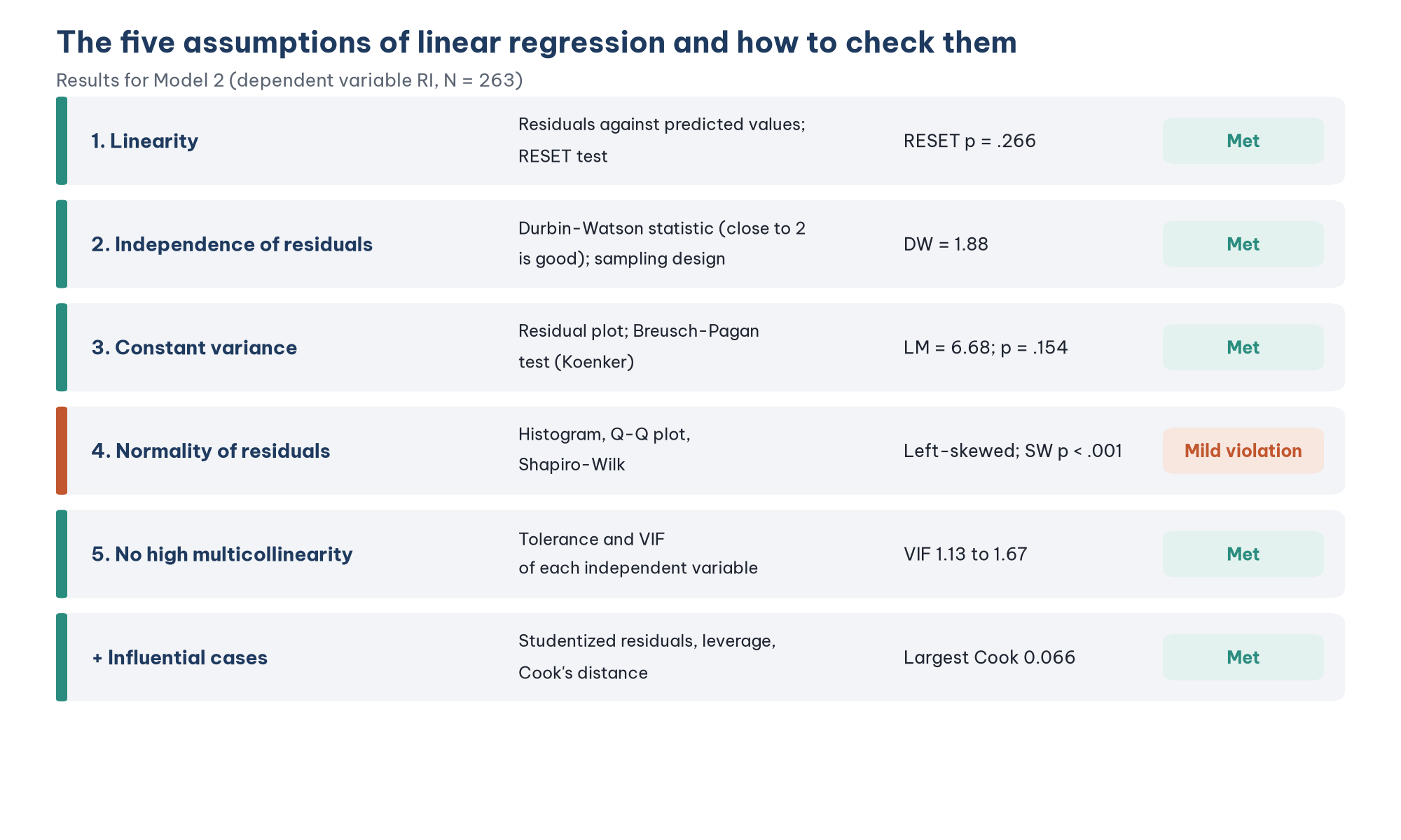
One point is often misunderstood: the assumptions are about the residuals (the errors of the model), not about the variables. Williams et al. (2013) point out two common misconceptions: that the independent and dependent variables must be normally distributed, and that multicollinearity is an assumption. In fact, regression does not require normally distributed variables. Multicollinearity is not an assumption but a problem in the data that inflates the standard errors.
Each assumption affects a different part of the results (Table 1).
2. Save the predicted values and residuals
In the Regression dialog (Post 14), click Save... and tick both boxes (Figure 2).
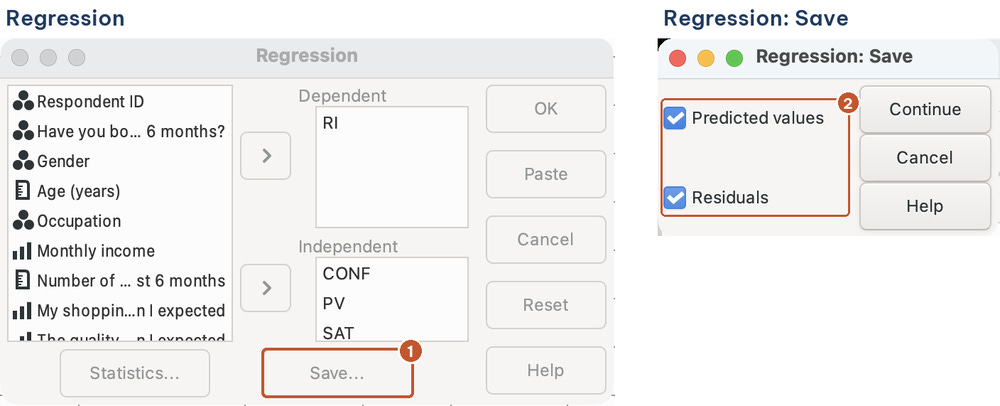
This is the biggest limitation of PSPP for checking assumptions. SPSS can also save standardized residuals, studentized residuals, Cook's distance, leverage and Mahalanobis distance, and has a Plots button that draws the residual plots for you. PSPP 2.1.2 has none of these options, and its Statistics dialog has no Durbin-Watson option either. The syntax file computes all of them.
The syntax file works on a copy of the data that keeps only the 263 responses with all five variables, so every statistic is based on the same responses as the model:
DATASET NAME MAIN.
DATASET COPY REG.
DATASET ACTIVATE REG.
SELECT IF NMISS(CONF, PV, SAT, TRU, RI) = 0.
REGRESSION /VARIABLES=CONF PV SAT TRU /DEPENDENT=RI /METHOD=ENTER
  /STATISTICS=COEFF R ANOVA TOL /SAVE=PRED RESID.
RENAME VARIABLES (PRED1 = PREDICTED) (RES1 = RESIDUAL).
PSPP names the two new variables PRED1 and RES1. The RENAME VARIABLES command gives them clearer names. Next, the standardized residual (ZRESID) is computed as the residual divided by the standard error of the estimate, the same way SPSS computes it:
COMPUTE RES_SQ = RESIDUAL ** 2.
AGGREGATE /OUTFILE=* MODE=ADDVARIABLES /SSE = SUM(RES_SQ) /N_REG = N(RESIDUAL)
  /M_PRED = MEAN(PREDICTED) /SD_PRED = SD(PREDICTED).
COMPUTE ZRESID = RESIDUAL / SQRT(SSE / (N_REG - 5)).
COMPUTE ZPRED = (PREDICTED - M_PRED) / SD_PRED.
AGGREGATE with MODE=ADDVARIABLES computes the sum of squared residuals (SSE) over all responses and attaches that value to every response. The number 5 is the number of parameters in the model: 4 coefficients and the constant.
3. Check multicollinearity
Multicollinearity occurs when the independent variables are too highly correlated with each other. Two statistics in the Coefficients table (with /STATISTICS=TOL) measure this problem:
Tolerance = 1 − *R*², where *R*² is the R-square obtained when that independent variable is regressed on the other independent variables. A small tolerance means that the variable is almost fully explained by the others.
VIF (variance inflation factor) = 1 / Tolerance. It tells you how many times the variance of the coefficient is "inflated" by multicollinearity.
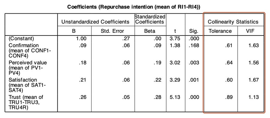
Hair et al. (2019) use the common cut-off of VIF above 10 (tolerance below .10) to flag serious multicollinearity, and many authors use the stricter cut-off of 5. The largest VIF in Model 2 is 1.67 (SAT), far below both cut-offs. In other words, the standard error of the SAT coefficient is about 1.3 times (the square root of 1.67) as large as it would be if SAT were completely uncorrelated with the other independent variables. Multicollinearity is not a problem here, as the correlation matrix in Post 13, "Pearson Correlation in PSPP (SPSS)" already suggested.
4. Check linearity
The model assumes that the relationship between the independent variables and RI is a straight line. There are two ways to check this.
With a plot. Plot the standardized residuals against the standardized predicted values:
GRAPH /SCATTERPLOT(BIVAR)=ZPRED WITH ZRESID.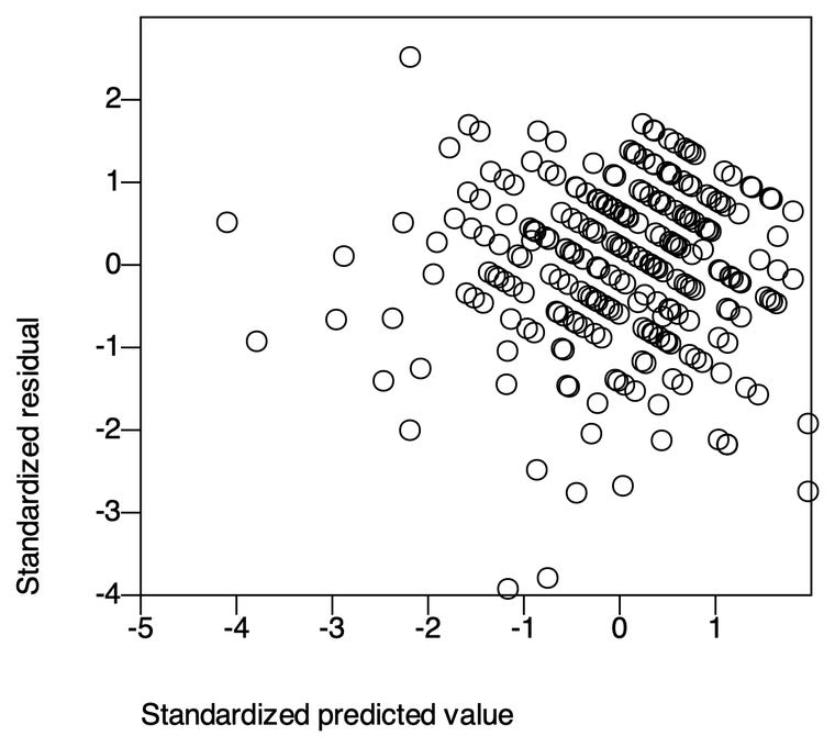
If the relationship is linear, the points are scattered randomly around the 0 line and do not form a U shape or an inverted U. The plot of the sample data meets this requirement. You will notice that the points line up along parallel diagonal lines. This is not a sign of a violation: RI can take only discrete values such as 3.00, 3.25 and 3.50, so the responses with the same RI value fall on the same diagonal line with a slope of −1.
With the RESET test (Ramsey, 1969). Add the square of the predicted value to the model. If the relationship really is linear, this extra variable explains nothing more:
COMPUTE PRED_SQ = PREDICTED ** 2.
REGRESSION /VARIABLES=CONF PV SAT TRU PRED_SQ /DEPENDENT=RI /METHOD=ENTER /STATISTICS=COEFF.
The coefficient of PRED_SQ has t = −1.11 and p = .266, which is not significant. The linearity assumption is met.
5. Check the independence of the residuals
The residuals of the responses must be independent of each other. This assumption is mainly ensured by the research design: each respondent answers once, independently of the others. It is violated when the data have a group structure (several employees from the same store) or a time structure (the same person surveyed several times).
The Durbin-Watson statistic (Durbin & Watson, 1951) tests the autocorrelation between the residuals of adjacent responses:
DW = sum of (e(i) − e(i−1))² / sum of e(i)²
where e(i) is the residual of response i. DW ranges from 0 to 4. A DW close to 2 means there is no autocorrelation. Field (2024) suggests that values below 1 or above 3 are cause for concern, and that the closer the value is to 2, the better. PSPP has no Durbin-Watson option, but the formula above can be computed with the LAG function:
SORT CASES BY ID.
COMPUTE DIFF_SQ = (RESIDUAL - LAG(RESIDUAL)) ** 2.
AGGREGATE /OUTFILE=* MODE=ADDVARIABLES /SUM_DIFF_SQ = SUM(DIFF_SQ).
COMPUTE DW = SUM_DIFF_SQ / SSE.
LAG(RESIDUAL) takes the residual of the previous response. The result: DW = 1.877, very close to 2.
Be clear about what this number means: DW depends on the order of the responses in the file. In cross-sectional survey data, the order of the responses (by ID, that is, the order in which they came in) usually has no special meaning, so DW only checks a very narrow kind of dependence: whether people who answered close together in time have similar residuals. DW is mainly useful for time-series data. For a survey, describe how the sample was drawn to show independence, and report DW as a supplementary check.
6. Check constant variance
The variance of the residuals must be the same at every level of the predicted values (homoscedasticity). When the variance changes (heteroscedasticity), the residual plot has a funnel shape: the points spread wide at one end and narrow at the other.
The plot in Figure 4 shows no clear funnel. For a more objective conclusion, use the Breusch-Pagan test (Breusch & Pagan, 1979), in the version of Koenker (1981), which is more robust when the residuals are not normal. The idea of the test: if the variance is constant, the independent variables cannot predict the size of the squared residuals. In PSPP:
REGRESSION /VARIABLES=CONF PV SAT TRU /DEPENDENT=RES_SQ /METHOD=ENTER /STATISTICS=R ANOVA.The test statistic is LM = N x R*² of this auxiliary regression, which follows a chi-square distribution with degrees of freedom equal to the number of independent variables. The auxiliary regression has R*² = 2.80 / 110.22 = 0.0254, so **LM = 263 x 0.0254 = 6.68, with 4 degrees of freedom, p = .154. The constant-variance hypothesis is not rejected. The F test of the auxiliary regression itself gives the same conclusion (F(4, 258) = 1.68, p = .155).
7. Check the normality of the residuals
EXAMINE VARIABLES=ZRESID /PLOT=HISTOGRAM NPPLOT /STATISTICS=DESCRIPTIVES EXTREME(5) /ID=ID.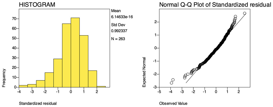
This is the only assumption that is violated. The residuals have a skewness of −0.81 and a kurtosis of 1.23. The Shapiro-Wilk test gives W = .96, p < .001 (PSPP prints the significance as 4.70E-006). In the Q-Q plot, most points lie close to the straight line, but at the lower end there are a few responses with large negative residuals: people whose repurchase intention is much lower than the model predicts. EXAMINE also draws a detrended Q-Q plot, which shows the same pattern.
Why are the residuals skewed to the left?
The cause lies in the data. RI has an upper limit of 5, and most respondents are already close to it (Post 9, "Descriptive Statistics in PSPP (SPSS)"). A customer with a predicted RI of 4.5 can have a positive residual of at most 0.5, but a negative residual as large as −3.5. This is the ceiling effect that is common with Likert scales when respondents lean strongly toward agreement.
Should you worry?
With a large sample, a violation of normality has little effect on regression. By the central limit theorem, the regression coefficients are approximately normally distributed when the sample is large enough, even if the residuals are not. Lumley et al. (2002) showed that with a few hundred observations, tests based on the normal distribution still give reliable results. The Shapiro-Wilk test works the other way: the larger the sample, the more easily it becomes significant for very small departures (Post 9).
As a check, the script check_python.py in the repository computes bootstrap confidence intervals (5,000 resamples), a method that does not assume normality (Table 2).
The two methods give almost identical intervals, and the conclusion about the significance of each variable does not change. The violation of normality does not affect the conclusions of the study.
8. Influential cases
A few unusual responses can pull the regression line toward them. Three statistics measure this:
Studentized residual: the residual divided by its own standard error for each response. An absolute value above 3 marks a response that the model predicts very poorly.
Leverage (h): how unusual a response is on the independent variables. A response whose combination of CONF, PV, SAT and TRU is far from the rest has high leverage. A common cut-off is 2(k + 1)/N = 10/263 = 0.038 (Hoaglin & Welsch, 1978).
Cook's distance (Cook, 1977): combines the residual and the leverage, and measures how much all the regression coefficients change when that response is removed. A Cook's distance above 1 is cause for concern; a more cautious cut-off is 4/N = 0.015.
PSPP can compute all three with the MATRIX command, using the algebraic formulas directly: leverage is the diagonal of the hat matrix H (the matrix of the independent variables, with a column of 1s for the constant, times the inverse of its cross-product matrix, times its transpose), and Cook's distance is e*²/(*p x MSE) x h/(1 − h)²:
MATRIX.
GET X /VARIABLES=CONF PV SAT TRU.
GET E /VARIABLES=RESIDUAL.
GET IDS /VARIABLES=ID.
COMPUTE N = NROW(X).
COMPUTE X1 = {MAKE(N, 1, 1), X}.
COMPUTE P = NCOL(X1).
COMPUTE H = DIAG(X1 * INV(T(X1) * X1) * T(X1)).
COMPUTE MSE = CSSQ(E) / (N - P).
COMPUTE COOK = (E &** 2 / (P * MSE)) &* (H &/ (1 - H) &** 2).
COMPUTE SRESID = E &/ SQRT(MSE * (1 - H)).
SAVE {IDS, H, COOK, SRESID} /OUTFILE='../data/influence.sav' /VARIABLES=ID LEVERAGE COOK SRESID.
END MATRIX.
The results agree with the statsmodels library in Python to three decimal places. The six responses with the largest Cook's distance:
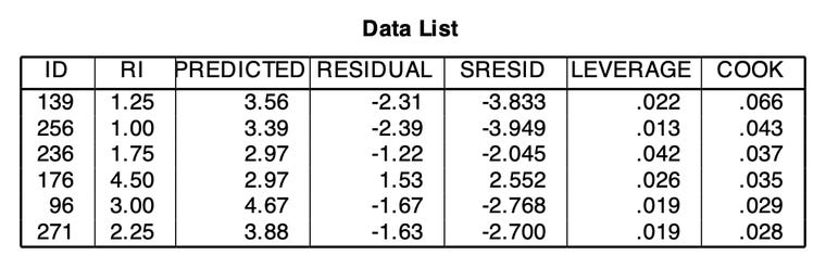
Table 3 summarizes the three criteria.
No response has a Cook's distance anywhere near 1. Responses 139 and 256 are customers who rate Marketplace X fairly well but have almost no intention of buying again. These are valid answers (they may have moved to another marketplace for reasons outside the model), not data errors, so they are not removed (Post 8, "Data Cleaning in PSPP (SPSS)").
Sensitivity analysis
To make sure the conclusions do not depend on a few responses, the syntax file runs the regression again without the 12 responses with a Cook's distance above 4/N (Table 4).
The size of the coefficients changes a little, but the conclusions about the hypotheses stay the same: PV, SAT and TRU still have significant positive effects, and CONF is still not significant at the .05 level. The main results are reported on all 263 responses, and the sensitivity analysis is mentioned as evidence that the results are robust.
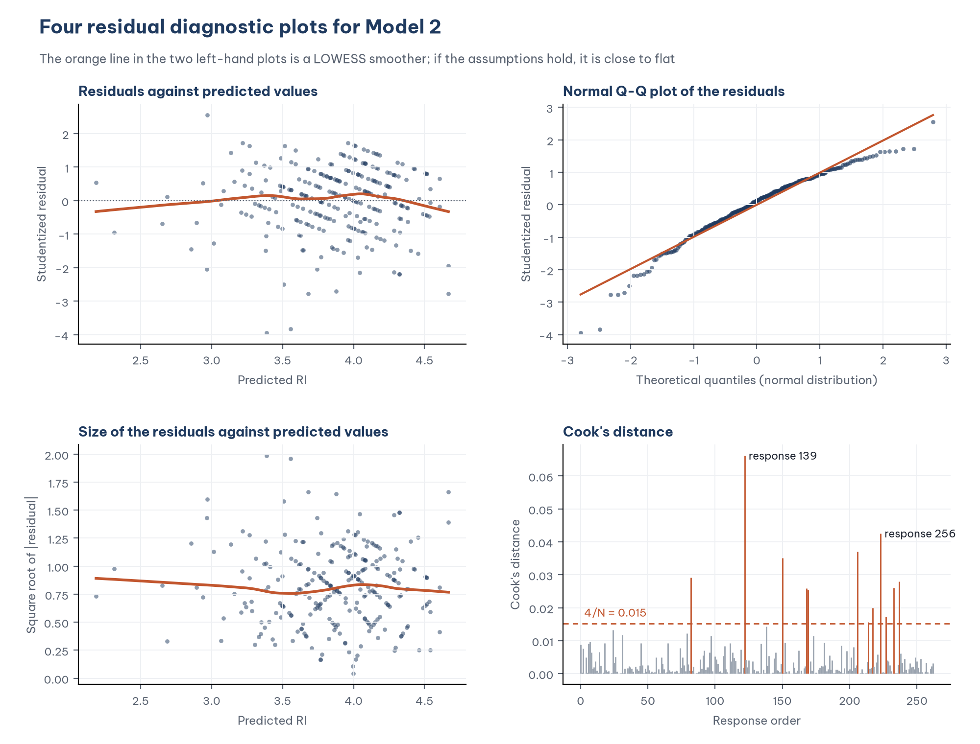
9. Four diagnostic plots in one figure
Statistical software such as R often combines four diagnostic plots in one figure. A short Python script draws a similar figure from the sample data, which is handy for the appendix of a thesis:
10. What to do when an assumption is violated
The sample data only mildly violate one assumption, but with real data you may meet more serious violations. Table 5 lists common remedies.
PSPP and base SPSS do not offer HC3 standard errors. As a comparison, the script check_python.py computes HC3 standard errors for Model 2: the standard errors barely change (for example, SAT: 0.064 against 0.064), and CONF is still not significant (p = .118). This is consistent with the result of the Breusch-Pagan test.
11. Report the results
The assumption checks are usually written up briefly in the results chapter, with the plots in an appendix. A sample paragraph:
"The assumptions of linear regression were checked for Model 2. VIF values from 1.13 to 1.67 indicate no multicollinearity. The RESET test (p = .266) and the residual plot showed no sign of a nonlinear relationship. The Breusch-Pagan test did not reject the assumption of constant variance (LM = 6.68, df = 4, p = .154). The Durbin-Watson statistic was 1.88. The residuals were mildly skewed to the left (skewness −0.81; Shapiro-Wilk p < .001), reflecting a ceiling effect in the Repurchase intention scale; with a sample of 263, bootstrap confidence intervals (5,000 resamples) were almost identical to the conventional intervals. No response had a Cook's distance above 0.07, and the conclusions about the hypotheses did not change when the 12 responses with a Cook's distance above 4/N were removed."
Five common mistakes
Checking the normality of the variables instead of the normality of the residuals.
Concluding that the model is "unusable" just because Shapiro-Wilk is significant in a large sample, without looking at the size of the departure and checking with the bootstrap.
Reporting Durbin-Watson as the only evidence of independence for cross-sectional survey data, when its value depends on the order of the responses.
Deleting responses with a large Cook's distance without checking why and without reporting the results before deletion.
Looking only at VIF < 10 and ignoring VIF values between 5 and 10, which are already enough to make the coefficients unstable in small samples.
Frequently asked questions
Do I need to check the assumptions for Model 1 (dependent variable SAT)?
Yes. Each regression equation has to be checked separately. The syntax file is written for Model 2; to check Model 1, change the dependent variable and the list of independent variables, and change the number of parameters (the number 5) to 3.
What is the difference between a P-P plot and a Q-Q plot?
A P-P plot (drawn by SPSS under the Plots button of Regression) compares cumulative probabilities and is sensitive to departures in the middle of the distribution. A Q-Q plot compares quantiles and is sensitive to departures in the tails. PSPP draws a Q-Q plot through the EXAMINE command. Both are acceptable in a report.
Why not use the Kolmogorov-Smirnov test for the residuals?
The Kolmogorov-Smirnov test is less sensitive than Shapiro-Wilk. PSPP prints the Shapiro-Wilk test in the EXAMINE command (the Tests of Normality table). Whichever test you use, with a large sample, read the result together with the plots and the skewness and kurtosis.
References
Breusch, T. S., & Pagan, A. R. (1979). A simple test for heteroscedasticity and random coefficient variation. Econometrica, 47(5), 1287–1294. https://doi.org/10.2307/1911963
Cook, R. D. (1977). Detection of influential observation in linear regression. Technometrics, 19(1), 15–18. https://doi.org/10.1080/00401706.1977.10489493
Durbin, J., & Watson, G. S. (1951). Testing for serial correlation in least squares regression. II. Biometrika, 38(1/2), 159–178. https://doi.org/10.2307/2332325
Field, A. (2024). Discovering statistics using IBM SPSS Statistics (6th ed.). SAGE Publications.
Free Software Foundation. (2026). GNU PSPP (Version 2.1.2) [Computer software]. https://www.gnu.org/software/pspp/
Hair, J. F., Black, W. C., Babin, B. J., & Anderson, R. E. (2019). Multivariate data analysis (8th ed.). Cengage Learning.
Hayes, A. F., & Cai, L. (2007). Using heteroskedasticity-consistent standard error estimators in OLS regression: An introduction and software implementation. Behavior Research Methods, 39(4), 709–722. https://doi.org/10.3758/BF03192961
Hoaglin, D. C., & Welsch, R. E. (1978). The hat matrix in regression and ANOVA. The American Statistician, 32(1), 17–22. https://doi.org/10.1080/00031305.1978.10479237
Koenker, R. (1981). A note on studentizing a test for heteroscedasticity. Journal of Econometrics, 17(1), 107–112. https://doi.org/10.1016/0304-4076(81)90062-2
Lumley, T., Diehr, P., Emerson, S., & Chen, L. (2002). The importance of the normality assumption in large public health data sets. Annual Review of Public Health, 23, 151–169. https://doi.org/10.1146/annurev.publhealth.23.100901.140546
Ramsey, J. B. (1969). Tests for specification errors in classical linear least-squares regression analysis. Journal of the Royal Statistical Society: Series B (Methodological), 31(2), 350–371. https://doi.org/10.1111/j.2517-6161.1969.tb00796.x
Williams, M. N., Grajales, C. A. G., & Kurkiewicz, D. (2013). Assumptions of multiple regression: Correcting two misconceptions. Practical Assessment, Research, and Evaluation, 18(11). https://doi.org/10.7275/55hn-wk47
Discussion about this post