Predictive Power in SmartPLS 4: Q²predict, PLSpredict and CVPAT
Set up PLSpredict, read Q²predict, compare RMSE with the linear model and run CVPAT to test out-of-sample prediction of a PLS-SEM model


Key takeaways
R² is in-sample explanatory power; PLSpredict measures how well the model predicts respondents who were not used to estimate it.
Read PLSpredict in two steps: Q²predict above 0 for every indicator, then compare PLS-SEM RMSE with the linear model (LM) benchmark.
The Marketplace X model has Q²predict from 0.085 to 0.213 and a lower RMSE than LM for all 12 indicators: high predictive power, though the RMSE gaps are small.
CVPAT tests whether the advantage is significant: overall yes (p < 0.001), but not for repurchase intention against LM (p = 0.137), and that result must be reported.
Use Fixed seed and report the number of folds, repetitions and prediction type, because the results depend on how the folds are split.
Post 37 showed that the Marketplace X model explains 31.8% of the variance of repurchase intention (R² = 0.318). R² measures in-sample explanatory power: the model is estimated and evaluated on the same data. This post asks a different question: if you apply the model to people who were not used to estimate it, how well does it predict their answers? This is step 5 of the structural model assessment of Hair et al. (2019): out-of-sample predictive power.
This post uses two tools built into SmartPLS 4:
PLSpredict (Shmueli et al., 2016, 2019): computes Q²predict and the prediction errors RMSE and MAE for each indicator.
CVPAT (Liengaard et al., 2021; Sharma et al., 2023): tests whether the prediction error of PLS-SEM is significantly lower than that of a benchmark model.
Sample data and scripts. The data file and scripts for this post are in the research-data-analysis repository on GitHub (folder
data/andscripts/). Download the whole repository with Code > Download ZIP.
About the figures and numbers. The figures are real screenshots of SmartPLS 4.1.2.1 (Ringle et al., 2026; 30-day trial) for the model
marketplace-x-modelfrom Post 33, with casewise deletion on 254 respondents. The Student license does not include PLSpredict and CVPAT. The numbers in this post come from the SmartPLS report. SmartPLS lists constructs and indicators in alphabetical order (INTENT, SATISF, VALUE; PV, RI, SAT). Section 6 checks the results in R (scriptplspredict.Rin the repository'sscripts/folder, cSEM package).
1. Why not use the blindfolding Q²?
Predictive power used to be assessed with the Stone-Geisser Q² (Geisser, 1974; Stone, 1974), computed by the blindfolding procedure: part of the data points is omitted in turn, the model is re-estimated and the omitted points are predicted. Shmueli et al. (2016) showed that this Q² still uses information from the very observations being predicted when the model is estimated, so it is closer to in-sample explanatory power than to out-of-sample prediction. For this reason, Hair et al. (2019) recommend PLSpredict for step 5, as does the primer by Hair et al. (2022).
If earlier studies or your supervisor ask for the blindfolding Q², you can report it as well, but state clearly that it is the blindfolding Q² and that it does not replace PLSpredict.
2. How does PLSpredict work?
PLSpredict uses k-fold cross-validation:
Split the 254 respondents at random into 10 folds of about 25 respondents each.
Estimate the model on 9 folds (the training sample, about 229 respondents).
Predict the answers of the remaining fold (the holdout sample) from the exogenous constructs of the model.
Repeat steps 2 and 3 until every fold has served as the holdout sample once.
Repeat the whole procedure 10 times with different splits, then average.
The result is the out-of-sample prediction error for each indicator of the endogenous constructs (the constructs being predicted: VALUE, SATISF and INTENT). The indicators of CONFIRM and TRUST do not appear in the results, because these exogenous constructs are the predictors.
The error of PLS-SEM is compared with two benchmarks:
IA (indicator average): predicts every respondent with the mean of the indicator in the training sample. This is the simplest possible prediction. Q²predict = 1 - (sum of squared prediction errors of PLS-SEM) / (sum of squared prediction errors of IA). A Q²predict above 0 means that PLS-SEM predicts better than the mean.
LM (linear model): regresses each indicator of an endogenous construct on all indicators of the exogenous constructs, without the structure of the model. This is a harder benchmark: PLS-SEM must predict at least as well as LM for the theoretical structure to add predictive value.
Two error measures:
RMSE (root mean squared error): penalizes large errors more heavily. Used by default.
MAE (mean absolute error): used when the distribution of the prediction errors is highly skewed (Shmueli et al., 2019). You can view this distribution under Histograms > PLS-SEM MV error histogram in the report.
3. Running PLSpredict in SmartPLS 4
Step 1. Open the model marketplace-x-model in the project Marketplace X. Choose the menu Calculate > PLSpredict / CVPAT.
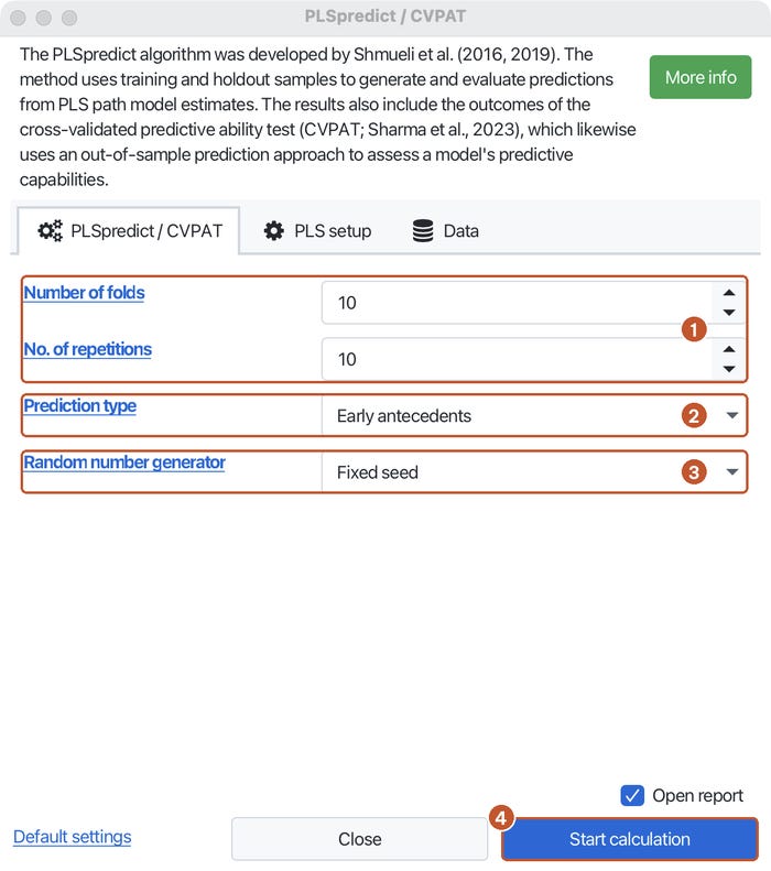
Step 2. On the PLSpredict / CVPAT tab of the dialog, check four settings (Figure 1):
Number of folds: 10.
No. of repetitions: 10.
Prediction type: Early antecedents, that is, predict from the first exogenous constructs of the path chain.
Random number generator: Fixed seed, so that a rerun gives the same results. With Random seed, the numbers vary slightly from run to run.
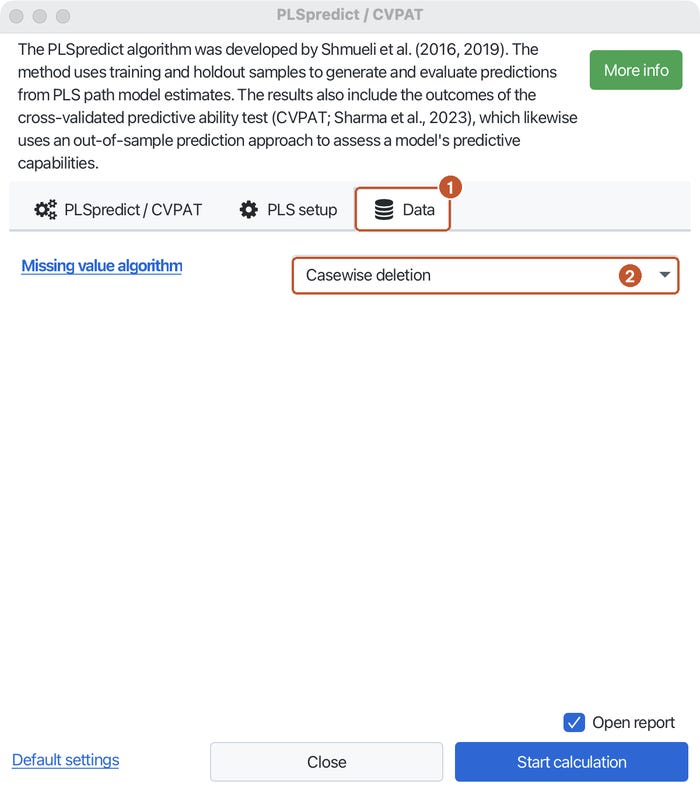
Step 3. Open the Data tab and set Missing value algorithm to Casewise deletion, as in the previous posts (Figure 2).
Step 4. Click Start calculation. With 10 folds and 10 repetitions, SmartPLS estimates the model 100 times, so it takes a few seconds.
Sample size in each fold. Each training sample contains only about 90% of the respondents. With small samples, use fewer folds (for example 5) so that the training sample does not become too small (Shmueli et al., 2019). With 254 respondents, 10 folds are appropriate.
4. Reading the PLSpredict results
Q²predict and RMSE of each indicator
Step 5. In the report, open Final results > PLSpredict MV summary > Overview (Figure 3).
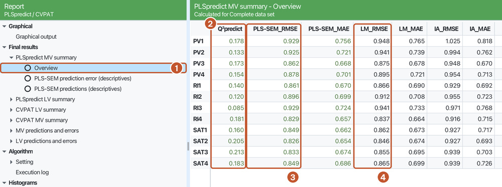
Shmueli et al. (2019) propose reading the results in two steps:
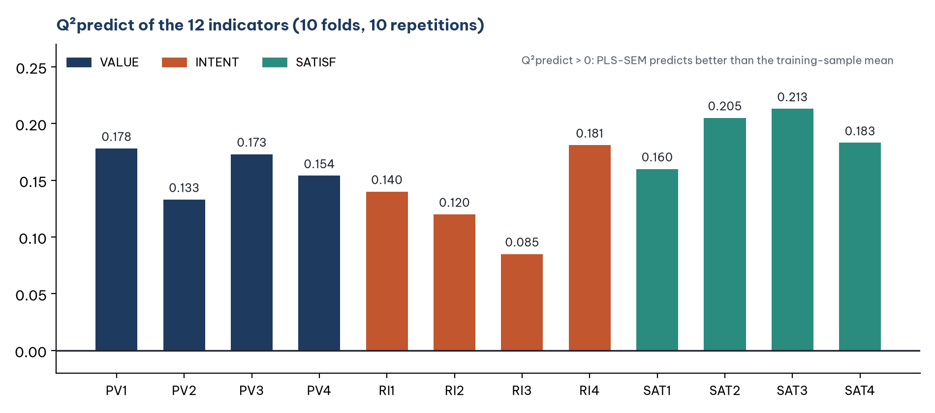
Check Q²predict. If the Q²predict of an indicator is above 0, PLS-SEM predicts better than IA. If Q²predict is 0 or below, the model has no predictive power for that indicator, and the assessment stops there.
Compare the RMSE of PLS-SEM with LM for the indicators of the key endogenous construct (here all 12 indicators are considered):
All indicators have a lower PLS-SEM RMSE than LM: high predictive power.
The majority are lower: medium predictive power.
A minority are lower: low predictive power.
None are lower: the model lacks predictive power.
Step 1 for the Marketplace X model: the Q²predict of the 12 indicators ranges from 0.085 (RI3) to 0.213 (SAT3), all above 0 (Figure 4).
Step 2: the PLS-SEM RMSE is lower than LM for all 12 indicators (Figure 5). MAE is also lower than LM for all 12 indicators (columns PLS-SEM_MAE and LM_MAE in Figure 3), so RMSE and MAE lead to the same conclusion.
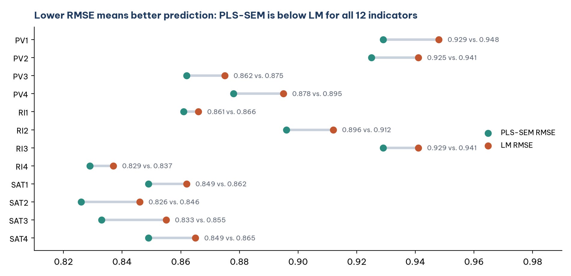
Conclusion following Shmueli et al. (2019): the Marketplace X model has high out-of-sample predictive power. Two further points should be read alongside this:
The RMSE differences are very small, from 0.005 (RI1) to 0.022 (SAT3). PLS-SEM beats LM for every indicator, but not by much.
Q²predict is low to moderate. The Q²predict of 0.085 for RI3 means that, compared with predicting by the mean, the squared error drops by only about 8.5%. Repurchase intention remains hard to predict from CONFIRM and TRUST, in line with the weak to moderate R² of Post 37.
Q²predict of the latent variables
Step 6. Open PLSpredict LV summary > PLS-SEM (Figure 6).
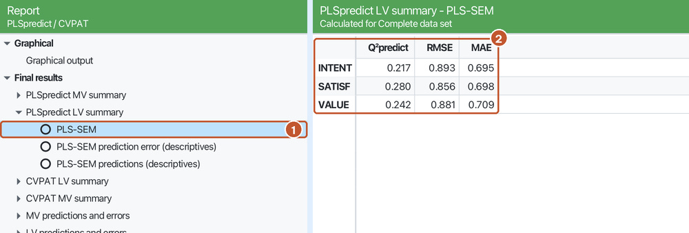
The Q²predict of the latent variables is lower than R², most clearly for SATISF (0.280 versus 0.399) and INTENT (0.217 versus 0.318). There are two reasons: Q²predict is computed on respondents outside the estimation sample, and with Early antecedents each construct is predicted only from the exogenous constructs (CONFIRM; plus TRUST for INTENT), not from the actual scores of VALUE and SATISF. This drop is normal, not an error.
Shmueli et al. (2019) recommend assessing predictive power on the indicators (the MV table), because users of the model predict actual answers, not latent variable scores. Use the LV table for reference.
5. The CVPAT test
PLSpredict tells you whether PLS-SEM has a lower error, but not whether the difference is statistically significant or just due to chance. CVPAT (cross-validated predictive ability test) answers this question (Liengaard et al., 2021). For each endogenous construct, CVPAT computes the average loss (the average squared prediction error) of PLS-SEM and of the benchmark, then runs a t test on the difference. A negative and significant difference means that PLS-SEM predicts better than the benchmark (Sharma et al., 2023).
Against the mean (IA)
Step 7. Open CVPAT LV summary > PLS-SEM vs. Indicator average (IA) (Figure 7).
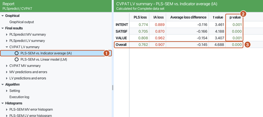
The loss difference is negative for all three constructs (−0.116 to −0.166), with p from 0.000 to 0.001. For the whole model: PLS-SEM loss 0.762, IA loss 0.907, difference −0.145, t = 4.688, p < 0.001. PLS-SEM predicts significantly better than the mean, consistent with Q²predict above 0 in Section 4.
Against the linear model (LM)
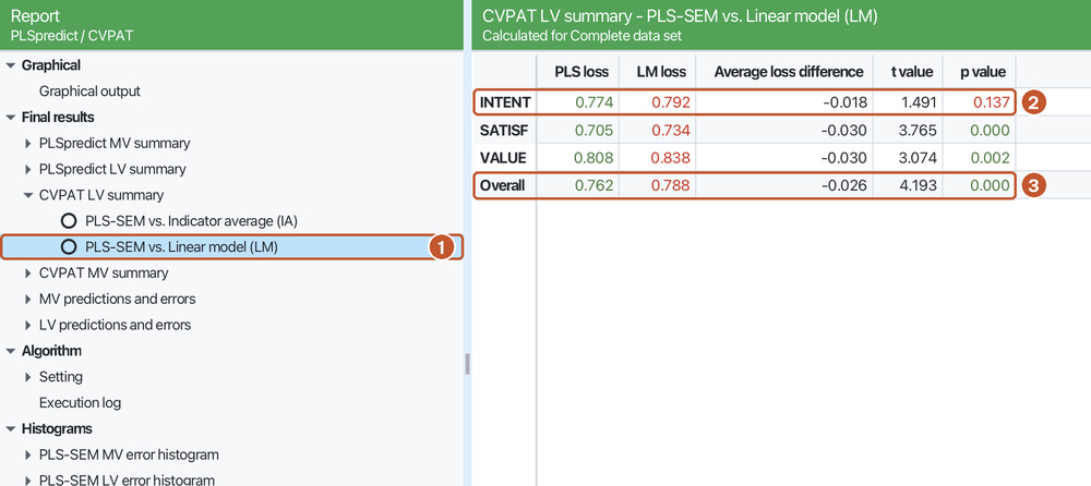
Step 8. Open CVPAT LV summary > PLS-SEM vs. Linear model (LM) (Figure 8).
Reading the results:
Whole model: PLS-SEM predicts significantly better than LM (t = 4.193, p < 0.001).
VALUE and SATISF: PLS-SEM is significantly better than LM (p = 0.002 and p < 0.001).
Repurchase intention (INTENT): the PLS-SEM loss is lower than the LM loss (0.774 versus 0.792), but the difference is not statistically significant (t = 1.491, p = 0.137). This p value is two-tailed; the one-tailed p would be about 0.069, still above 0.05.
This result complements, rather than contradicts, PLSpredict. PLSpredict shows a lower PLS-SEM RMSE than LM for all four indicators RI1 to RI4; CVPAT shows that, for INTENT, this advantage is so small that chance cannot be ruled out. Report it exactly that way: for the most important construct of the model, the theoretical structure does not yet predict clearly better than a direct linear regression on the indicators.
6. Checking in R
The script plspredict.R runs the same model with the predict() function of the cSEM package: 10 folds, 10 repetitions, LM as the benchmark, regular PLS-SEM (no PLSc correction), 254 respondents. Because the random fold assignment differs from SmartPLS, the results agree only approximately:
Q²predict agrees to the second decimal place, for example PV1 0.177 (R) versus 0.178 (SmartPLS), RI3 0.085 versus 0.085, SAT3 0.211 versus 0.213.
The PLS-SEM RMSE is almost identical, for example PV1 0.929 versus 0.929.
The LM RMSE in cSEM is larger than in SmartPLS (for example PV1 0.986 versus 0.948), so the gap between PLS-SEM and LM is larger in cSEM. We have not identified which setting of the two programs causes this difference. Still, the conclusion is the same: the PLS-SEM RMSE is lower than LM for all 12 indicators.
The R values above come from the run saved in plspredict.csv. In cSEM 0.7.1, set.seed() does not fix the folds of predict() with more than one repetition, so rerunning the script gives values that differ in the third decimal place; the conclusions do not change.
This post uses the SmartPLS numbers. If you use other software, report the software, the number of folds, the number of repetitions and how random numbers were generated.
7. Reporting the results
Out-of-sample predictive power was assessed with PLSpredict (Shmueli et al., 2019) using 10 folds and 10 repetitions. The Q²predict values of the 12 indicators of the three endogenous constructs were all above 0 (0.085 to 0.213), and the PLS-SEM RMSE was lower than that of the linear model for all 12 indicators, indicating high predictive power according to the criteria of Shmueli et al. (2019). However, the RMSE differences were small (0.005 to 0.022). The CVPAT test (Sharma et al., 2023) showed that PLS-SEM predicted better than the indicator average (loss difference −0.145, t = 4.688, p < 0.001) and better than the linear model (−0.026, t = 4.193, p < 0.001) at the overall model level. For repurchase intention, however, PLS-SEM did not predict significantly better than the linear model (t = 1.491, p = 0.137).
In a thesis table, present Q²predict and the RMSE (or MAE) of PLS-SEM and of LM for each indicator, as in the table in Section 4, together with the CVPAT table, and note the number of folds, the number of repetitions and the prediction type.
Five common mistakes
Reporting the blindfolding Q² as evidence of out-of-sample prediction. This Q² is closer to in-sample explanatory power (Shmueli et al., 2016).
Reporting only that Q²predict is above 0 and concluding "good prediction". Q²predict above 0 is only the minimum requirement; you still need the comparison with LM.
Comparing the PLS-SEM RMSE with the IA RMSE. The benchmark in step 2 is LM. IA is already used in Q²predict.
Ignoring a non-significant CVPAT result. The INTENT result in this post must be reported and discussed, not just the Overall row.
Not reporting the settings. The results vary with the fold assignment; without the number of folds, the number of repetitions and the seed, readers cannot check the results.
Frequently asked questions
What Q²predict counts as high?
Shmueli et al. (2019) give no threshold for Q²predict other than being above 0; the main assessment rests on the comparison with LM. To describe its size, you can use the rule of thumb in Hair et al. (2019): Q² values above 0, 0.25 and 0.50 indicate small, medium and large predictive relevance. By this rule, the Q²predict values of the indicators in the Marketplace X model are small.
Why do only the indicators of VALUE, SATISF and INTENT appear in the results?
PLSpredict predicts the endogenous constructs from the exogenous constructs. CONFIRM and TRUST are exogenous, so their indicators are inputs, not prediction targets.
My results differ by a few thousandths from my previous run. Why?
Check the Random number generator setting. With Random seed, each run splits the folds differently, so the numbers vary slightly. Choose Fixed seed to get the same results when you rerun.
Does a non-significant CVPAT result mean the model is rejected?
No. CVPAT assesses predictive power; it does not test causal hypotheses. Hypotheses H1 to H7 are tested with bootstrapping in Post 39. Put the CVPAT result in the discussion and limitations: the model explains the relationships between the constructs, but its ability to predict repurchase intention does not yet clearly exceed that of a simple regression model.
References
Geisser, S. (1974). A predictive approach to the random effect model. Biometrika, 61(1), 101–107. https://doi.org/10.1093/biomet/61.1.101
Hair, J. F., Hult, G. T. M., Ringle, C. M., & Sarstedt, M. (2022). A primer on partial least squares structural equation modeling (PLS-SEM) (3rd ed.). SAGE Publications.
Hair, J. F., Risher, J. J., Sarstedt, M., & Ringle, C. M. (2019). When to use and how to report the results of PLS-SEM. European Business Review, 31(1), 2–24. https://doi.org/10.1108/EBR-11-2018-0203
Liengaard, B. D., Sharma, P. N., Hult, G. T. M., Jensen, M. B., Sarstedt, M., Hair, J. F., & Ringle, C. M. (2021). Prediction: Coveted, yet forsaken? Introducing a cross-validated predictive ability test in partial least squares path modeling. Decision Sciences, 52(2), 362–392. https://doi.org/10.1111/deci.12445
Ringle, C. M., Wende, S., & Becker, J.-M. (2026). SmartPLS 4 (Version 4.1.2.1) [Computer software]. SmartPLS GmbH. https://www.smartpls.com
Sharma, P. N., Liengaard, B. D., Hair, J. F., Sarstedt, M., & Ringle, C. M. (2023). Predictive model assessment and selection in composite-based modeling using PLS-SEM: Extensions and guidelines for using CVPAT. European Journal of Marketing, 57(6), 1662–1677. https://doi.org/10.1108/EJM-08-2020-0636
Shmueli, G., Ray, S., Velasquez Estrada, J. M., & Chatla, S. B. (2016). The elephant in the room: Predictive performance of PLS models. Journal of Business Research, 69(10), 4552–4564. https://doi.org/10.1016/j.jbusres.2016.03.049
Shmueli, G., Sarstedt, M., Hair, J. F., Cheah, J.-H., Ting, H., Vaithilingam, S., & Ringle, C. M. (2019). Predictive model assessment in PLS-SEM: Guidelines for using PLSpredict. European Journal of Marketing, 53(11), 2322–2347. https://doi.org/10.1108/EJM-02-2019-0189
Stone, M. (1974). Cross-validatory choice and assessment of statistical predictions. Journal of the Royal Statistical Society: Series B (Methodological), 36(2), 111–147. https://doi.org/10.1111/j.2517-6161.1974.tb00994.x
Discussion about this post