Reflective Measurement Model in SmartPLS 4: Loadings, Reliability and AVE
Check outer loadings, Cronbach’s alpha, rho_a, rho_c and AVE step by step, and see why PLS-SEM reports a higher AVE than CB-SEM


Key takeaways
A reflective measurement model is evaluated in order: outer loadings, internal consistency reliability, convergent validity (AVE), then discriminant validity.
Loadings should reach 0.708; an indicator below that is not removed automatically, and only one below 0.40 is always removed.
Report Cronbach's alpha, rho_a and rho_c together: alpha tends to be low, rho_c tends to be high and rho_a lies in between; values above 0.95 signal redundant indicators.
On the Marketplace X data all 20 loadings range from 0.754 to 0.876 and AVE from 0.612 to 0.682, so every criterion is met.
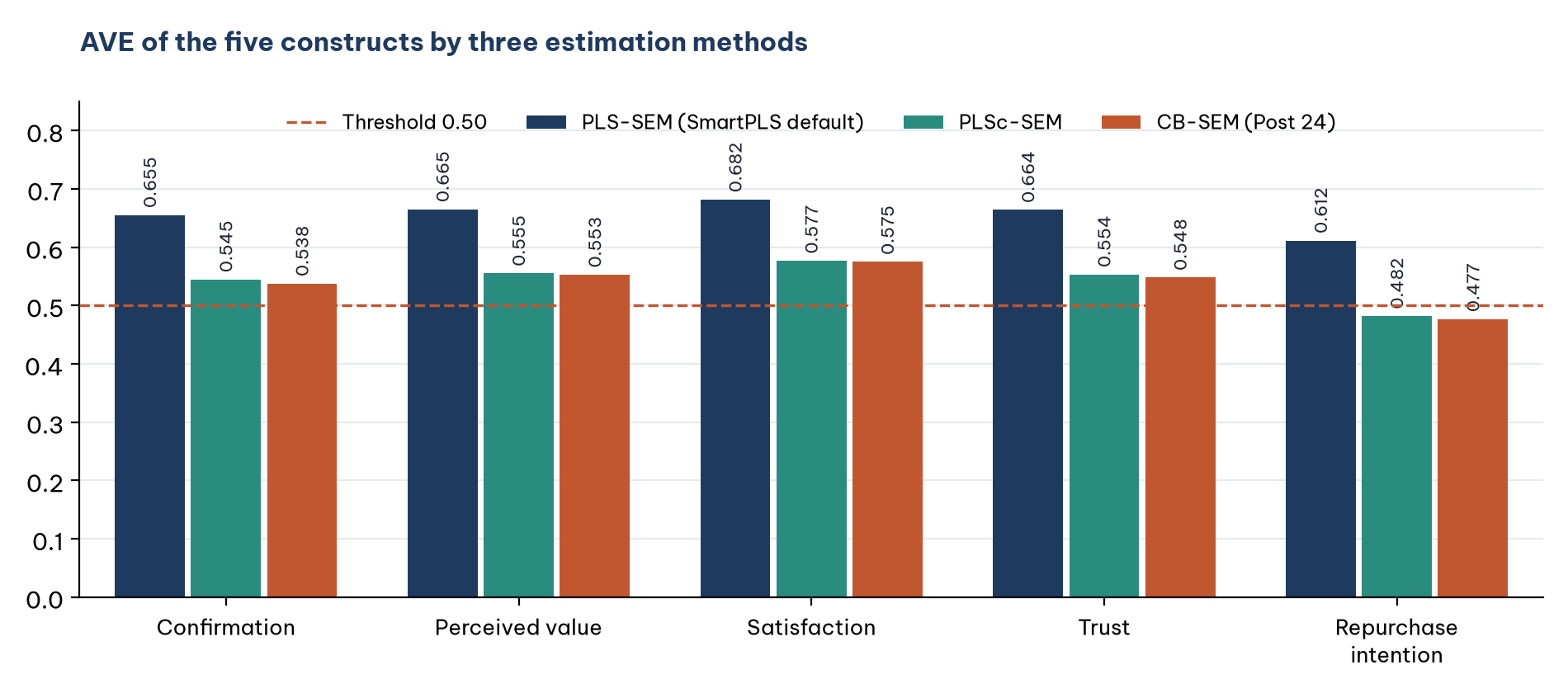
PLS-SEM inflates loadings: the AVE of Repurchase intention is 0.612 here, 0.482 with consistent PLS and 0.477 in CB-SEM. Choose the method for its rationale, never for its results.
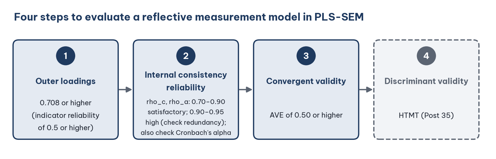
Post 33 drew the Marketplace X model and ran the PLS-SEM algorithm. Before reading the path coefficients, you need to make sure that the scales measure their constructs correctly and consistently. For a reflective measurement model, this takes three steps: check the outer loadings, the internal consistency reliability and the convergent validity (Hair et al., 2019). The fourth step, discriminant validity, is the topic of Post 35.
The results on the Marketplace X data raise one point worth discussing: the AVE of the Repurchase intention scale is 0.612, above the threshold, whereas Post 24 (CB-SEM) gave 0.477, below it. Section 5 explains why and how to report it.
Sample data and scripts. The data file and scripts for this post are in the research-data-analysis repository on GitHub (folder
data/andscripts/). Download the whole repository with Code > Download ZIP.
About the figures and numbers. The figures are real screenshots of the SmartPLS 4.1.2.1 report (Ringle et al., 2026; 30-day trial) for the model
marketplace-x-modelfrom Post 33, run with casewise deletion on 254 respondents, taken in November 2026. Every number was checked with the cSEM 0.7.1 package (Rademaker & Schuberth, 2026), scriptevaluate_measurement.Rin the repository'sscripts/folder, and matches SmartPLS to the third decimal place.
1. Open the results in SmartPLS
Open the report of the PLS-SEM algorithm (Post 33, Section 6). The two tables you need are in the Report pane on the left:
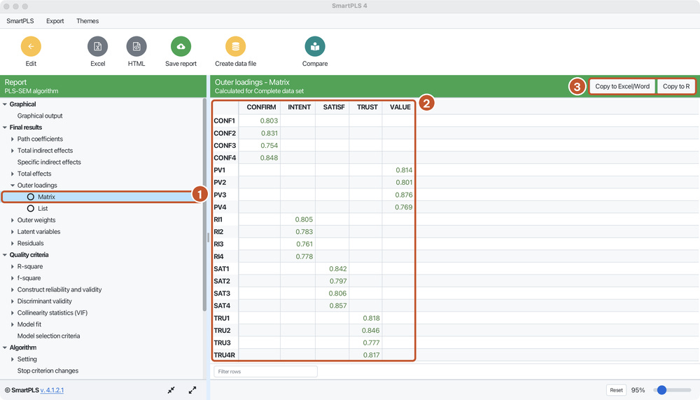
Step 1. In the Final results group, click the arrow next to Outer loadings, then choose Matrix (Figure 2).
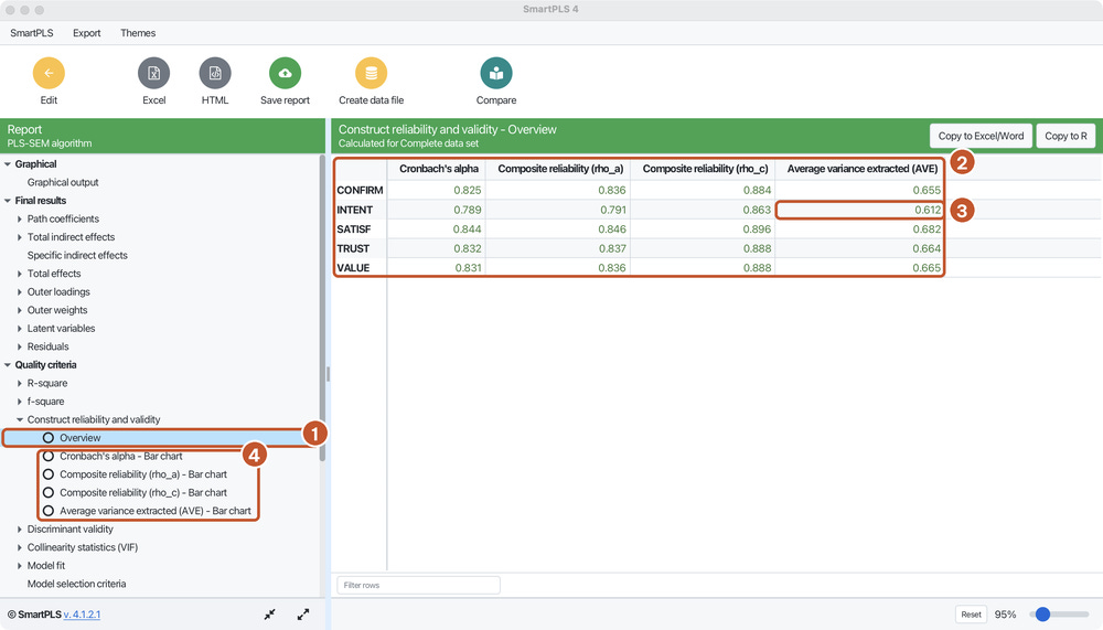
Step 2. In the Quality criteria group, click the arrow next to Construct reliability and validity, then choose Overview (Figure 3).
Three things to note when reading the report:
The line Calculated for Complete data set at the top of each table tells you that the results are based on the complete responses (casewise deletion, Post 33).
SmartPLS sorts constructs and indicators alphabetically in these tables (CONFIRM, INTENT, SATISF, TRUST, VALUE), not in the order in which you drew them. The tables in this post follow the same order.
The Copy to Excel/Word and Copy to R buttons copy the whole table so you can paste it into your thesis without retyping. According to the license comparison, the Student license cannot copy or export reports (SmartPLS GmbH, n.d.).
2. Step 1: Outer loadings
The outer loading is the correlation between an indicator and its latent variable. The squared loading is the indicator reliability: the share of the indicator's variance explained by the construct.
Threshold: loadings of 0.708 or higher, because the squared loading is then 0.5: the construct explains at least half of the indicator's variance (Hair et al., 2019). An indicator with a loading below 0.708 is not removed automatically (Hair et al., 2022):
Below 0.40: remove the indicator.
From 0.40 to below 0.708: remove it only if removal brings rho_c or AVE above the threshold, and does not remove an important aspect of the construct's content.
Result: all 20 indicators have loadings from 0.754 (CONF3) to 0.876 (PV3), all above 0.708. No indicator needs to be considered for removal. TRU4R (the reverse-worded item recoded in Post 10) has a loading of 0.817: the recoding went in the right direction; had it not been recoded, its loading would be negative.
Testing the significance of the loadings requires bootstrapping, covered in Post 39.
3. Step 2: Internal consistency reliability
SmartPLS reports three reliability criteria (Figure 3):
Cronbach's alpha (Cronbach, 1951): assumes that every indicator contributes equally (Post 11). When loadings differ, alpha is usually lower than the true reliability.
Composite reliability (rho_c) (Jöreskog, 1971): uses the estimated loadings, so each indicator can contribute differently. This is the CR from Post 24, computed with the same formula. In PLS-SEM, rho_c is usually higher than the true reliability, because the loadings are inflated (Post 31).
Composite reliability (rho_a) (Dijkstra & Henseler, 2015): computed from the weights of the composite. Its value usually lies between alpha and rho_c, so it is regarded as a good compromise and the most reliable measure for PLS-SEM (Hair et al., 2019).
Thresholds (Hair et al., 2019):
Result: all three criteria of the five scales lie between 0.70 and 0.90: satisfactory. The order alpha below rho_a, rho_a below rho_c is as theory predicts. Cronbach's alpha here is close to Post 11 (for example CONFIRM 0.825 versus 0.824); the small difference arises because Post 11 used a different sample.
Computing rho_c by hand for the Repurchase intention scale
The formula is the same as in Post 24, with L the loading:
rho_c = (Sum of L)² / [(Sum of L)² + Sum of (1 - L²)]
Add the four loadings: 0.805 + 0.783 + 0.761 + 0.778 = 3.128 (from the unrounded loadings, 3.1277; the rounded values add to 3.127); squaring the unrounded sum 3.1277 gives 9.782 (squaring 3.128 itself would give 9.784).
Add the four error terms (1 - L²): 4 - (0.649 + 0.613 + 0.579 + 0.605) = 4 - 2.446 = 1.554.
Compute rho_c = 9.782 / (9.782 + 1.554) = 0.863, exactly as in SmartPLS.
4. Step 3: Convergent validity (AVE)
AVE (average variance extracted) is the mean of the squared loadings of the indicators in a scale (Fornell & Larcker, 1981). AVE tells you how much of the indicators' variance the construct explains on average.
Threshold: AVE of 0.50 or higher (Fornell & Larcker, 1981; Hair et al., 2019).
By hand for the Repurchase intention scale: AVE = (0.649 + 0.613 + 0.579 + 0.605) / 4 = 2.446 / 4 = 0.612.
Result: the five scales have AVE from 0.612 to 0.682: convergent validity is established.
5. Why does the AVE of Repurchase intention differ from Post 24?
In Post 24, the CB-SEM CFA gave the Repurchase intention scale an AVE of 0.477, below the threshold. Here PLS-SEM gives 0.612. Same data, same four indicators, yet different conclusions. The reason lies in how the construct is understood (Post 31):
PLS-SEM treats the construct as a composite of its own indicators, which includes measurement error. Each indicator is part of the composite, so it correlates more strongly with it: the loadings are inflated, and so are AVE and rho_c.
Consistent PLS (PLSc) corrects this bias. With PLSc, the AVE of Repurchase intention is 0.482, close to the 0.477 from CB-SEM (Figure 4).
How should you report this?
If your thesis uses PLS-SEM: report the PLS-SEM results as SmartPLS gives them, because the thresholds in Sections 2 to 4 were proposed for these very criteria (Hair et al., 2019). The Repurchase intention scale meets every criterion.
Do not choose the method by its results. Switching from CB-SEM to PLS-SEM only to push AVE above 0.5 is not honest. The choice of PLS-SEM must rest on how the constructs are understood and on the research goal (Post 31).
If the constructs are understood as common factors (like the five constructs of the Marketplace X study) and you want less biased estimates, use PLSc, or state in the limitations that the AVE of Repurchase intention is close to the threshold once measurement error is corrected (0.482). This is the same honest reporting as in Post 24.
6. Reporting the results
The measurement model was evaluated following Hair et al. (2019). The loadings of the 20 indicators ranged from 0.754 to 0.876, all above the 0.708 threshold. The internal consistency reliability of the five scales was satisfactory: Cronbach's alpha ranged from 0.789 to 0.844, rho_a from 0.791 to 0.846 and rho_c from 0.863 to 0.896, all between 0.70 and 0.90. The average variance extracted (AVE) ranged from 0.612 to 0.682, above the 0.50 threshold, indicating convergent validity. When measurement error was corrected with consistent PLS, the AVE of the Repurchase intention scale was 0.482, close to the threshold; this point is noted in the limitations.
The table in your thesis should combine the loadings, alpha, rho_a, rho_c and AVE of each scale. Use the Copy to Excel/Word button to copy the tables from SmartPLS.
Five common mistakes
Removing an indicator only because its loading is below 0.708, without checking whether removal brings rho_c or AVE above the threshold, and without considering its content.
Reporting only Cronbach's alpha. In PLS-SEM, report rho_a and rho_c as well.
Assuming that a higher rho_c is always better. Above 0.95 signals redundant indicators or straight-lining.
Comparing PLS-SEM AVE directly with studies that used CB-SEM without noting the bias of PLS-SEM (Section 5).
Reading the results of an old run after changing the model. Every time you change the model, run the algorithm again before reading the tables.
Frequently asked questions
CONF3 has the lowest loading (0.754). Should I remove it to raise AVE?
No. CONF3 is above the 0.708 threshold, and the AVE of CONFIRM (0.655) is already met. Removing an indicator that meets the criteria only loses content from the scale.
How do rho_a and rho_c differ, and which should I report?
Report both, together with Cronbach's alpha, as in the table in Section 3. Alpha tends to be low and rho_c tends to be high in PLS-SEM, with rho_a in between (Hair et al., 2019). If all three meet the threshold, as in the Marketplace X data, the conclusion is robust.
Do I need to test the significance of the loadings?
Yes, with bootstrapping (Post 39). With loadings of 0.75 or higher on 254 respondents, they are almost certainly significant, but you should still report the test.
Are formative scales evaluated this way?
No. For formative scales, loadings, alpha and AVE do not have the meaning described above. Their evaluation (VIF, weights) is covered in Post 36.
References
Cronbach, L. J. (1951). Coefficient alpha and the internal structure of tests. Psychometrika, 16(3), 297–334. https://doi.org/10.1007/BF02310555
Dijkstra, T. K., & Henseler, J. (2015). Consistent partial least squares path modeling. MIS Quarterly, 39(2), 297–316. https://doi.org/10.25300/MISQ/2015/39.2.02
Fornell, C., & Larcker, D. F. (1981). Evaluating structural equation models with unobservable variables and measurement error. Journal of Marketing Research, 18(1), 39–50. https://doi.org/10.2307/3151312
Hair, J. F., Hult, G. T. M., Ringle, C. M., & Sarstedt, M. (2022). A primer on partial least squares structural equation modeling (PLS-SEM) (3rd ed.). SAGE Publications.
Hair, J. F., Risher, J. J., Sarstedt, M., & Ringle, C. M. (2019). When to use and how to report the results of PLS-SEM. European Business Review, 31(1), 2–24. https://doi.org/10.1108/EBR-11-2018-0203
Jöreskog, K. G. (1971). Statistical analysis of sets of congeneric tests. Psychometrika, 36(2), 109–133. https://doi.org/10.1007/BF02291393
Rademaker, M. E., & Schuberth, F. (2026). cSEM: Composite-based structural equation modeling (R package version 0.7.1) [Computer software]. https://CRAN.R-project.org/package=cSEM
Ringle, C. M., Wende, S., & Becker, J.-M. (2026). SmartPLS 4 (Version 4.1.2.1) [Computer software]. SmartPLS GmbH. https://www.smartpls.com
SmartPLS GmbH. (n.d.). Pricing and licenses. Retrieved November 6, 2026, from https://smartpls.com/pricing/
Discussion about this post