What Is SmartPLS? PLS-SEM vs CB-SEM and When to Use Each
Compare PLS-SEM and CB-SEM on the same data, from path coefficients and loadings to R², and choose the right method for your thesis


Key takeaways
CB-SEM treats a construct as a common factor; PLS-SEM treats it as a composite, a weighted sum of its items.
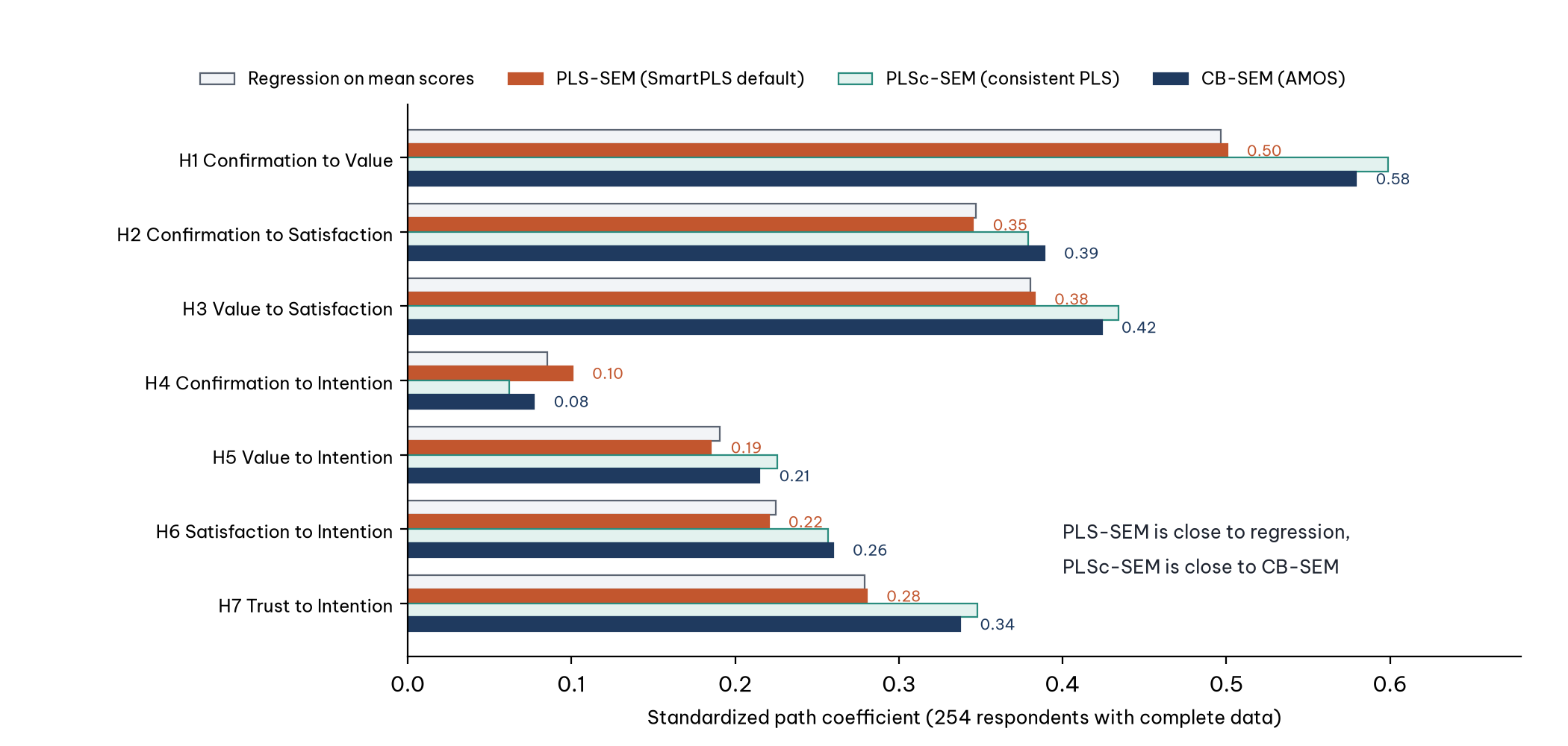
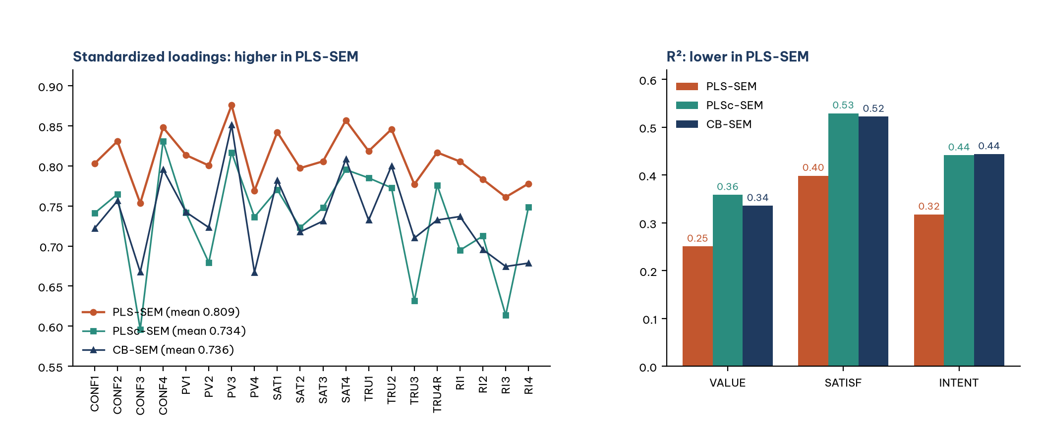
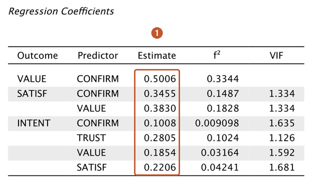
On the same data PLS-SEM gives smaller paths (H1: 0.501 against 0.579), lower R² and higher loadings than CB-SEM.
Consistent PLS (PLSc) corrects these biases and lands within 0.02 of CB-SEM.
Both methods reach the same conclusions about direction and significance; only the size of the coefficients differs.
A small sample or non-normal data is not a sufficient reason to choose PLS-SEM; justify the choice by the constructs and the research goal.
The AMOS posts (Post 19 to Post 30) estimated the Marketplace X model with CB-SEM. This post opens the SmartPLS series with the question every thesis committee asks: why did you choose PLS-SEM, or why not? Instead of just listing pros and cons, the post estimates the same model on the same data set in four ways and puts the results side by side.
Sample data and scripts. The data files and scripts for this post are in the research-data-analysis repository on GitHub (folder
data/andscripts/). Download the whole repository with Code > Download ZIP.
About the figures and numbers. The numbers were computed with the R packages cSEM 0.7.1 (Rademaker & Schuberth, 2026) and lavaan 0.7.3 (Rosseel, 2012), using the script
compare_pls_cbsem.Rin the repository, on the 254 respondents who answered all 20 items (marketplace_x_sem_complete.sav). The screenshots come from the Partial Least Squares SEM module of JASP 0.99.0 (JASP Team, 2026) on macOS; this module is built on the cSEM package, and its PLS-SEM estimates match the R results to the fourth decimal. There are no SmartPLS screenshots in this post.
1. What is SmartPLS?
SmartPLS is software for estimating structural equation models with partial least squares (PLS-SEM), developed by Christian M. Ringle, Sven Wende and Jan-Michael Becker since 2005. The current version is SmartPLS 4.1.2.1, released on 25 October 2026 (Ringle et al., 2026). Its main features:
Drag-and-drop interface: you draw the model with the mouse and read Excel, CSV and SPSS files directly.
The full PLS-SEM toolbox: bootstrapping, PLSpredict, multigroup analysis (MGA), IPMA, higher-order models and moderators. SmartPLS 4 also offers CB-SEM and regression.
Commercial license: there is a 30-day trial with all features and a free Student license with reduced functionality (CSV files only, at most 100 rows of data; see Post 32, "How to Install SmartPLS 4 and Find Your Way Around the Interface"). The SmartPLS release notes state that the Student license now includes basic CB-SEM functions and bootstrapping for CB-SEM.
Operating systems: Windows and macOS.
2. How does PLS-SEM differ from CB-SEM?
The core difference lies in how a construct is understood (Sarstedt et al., 2016):
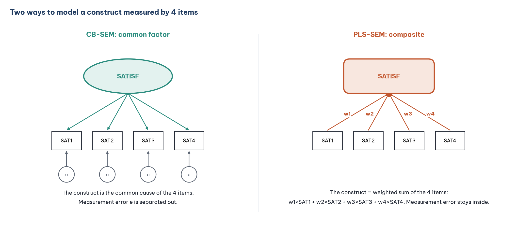
CB-SEM treats a construct as a common factor: satisfaction is the cause that makes respondents give high scores on SAT1 to SAT4; the rest of each item is measurement error and is separated out. The method estimates all parameters at once so that the covariance matrix implied by the model fits the data as closely as possible.
PLS-SEM treats a construct as a composite: a weighted sum of its four items. The algorithm alternates between two steps, finding a weight for each item and then running regressions between the composites, until the weights are stable (Wold, 1982; Hair et al., 2022). Its goal is to maximize the R² of the dependent constructs.
Because a composite also contains measurement error, PLS-SEM has two well-known biases when the construct really is a common factor (Dijkstra & Henseler, 2015):
Loadings are inflated, because each item is part of the composite itself.
Path coefficients and R² are attenuated, because measurement error dilutes the relationships between constructs, just as in a regression on mean scores (Post 19).
Consistent PLS (PLSc) corrects these two biases using the reliability of each construct, which gives estimates close to CB-SEM (Dijkstra & Henseler, 2015).
3. Comparison on the Marketplace X data
The model is the one from Post 26, "Structural Equation Model (SEM) in JASP": five constructs and seven hypotheses, H1 to H7. The data are the 254 respondents with complete answers, because cSEM and JASP require data without missing cells (how SmartPLS handles missing cells is covered in Post 33, "Importing Data and Drawing a Model in SmartPLS 4").
How to read the results:
PLS-SEM almost coincides with regression on mean scores: the path coefficients differ by at most 0.02. This makes sense: a composite with nearly equal weights is the mean score.
Compared with CB-SEM, PLS-SEM gives smaller path coefficients (for example H1: 0.501 versus 0.579; H7: 0.280 versus 0.338), lower R² (repurchase intention: 0.318 versus 0.444) and higher loadings (mean 0.809 versus 0.736). These are exactly the two biases described in Section 2.
PLSc-SEM is close to CB-SEM: the path coefficients differ by at most 0.02, and the mean loadings are almost equal.
The test conclusions are the same. Bootstrapping PLS-SEM with 5,000 samples: H4 is not significant (p = 0.086; 95% confidence interval [−0.017, 0.210]), and the other six hypotheses are significant, as in CB-SEM (H4: p = 0.443). The p values of PLS-SEM are smaller on some paths, for example H5: 0.007 versus 0.027.
The lesson: with reflective constructs such as those in the Marketplace X model, PLS-SEM and CB-SEM usually lead to the same conclusions about direction and significance, but the size of the coefficients differs in a systematic way. When you compare your results with earlier studies, check which method those studies used.
Estimating the model in JASP
You can reproduce the PLS-SEM column for free in JASP:
Open
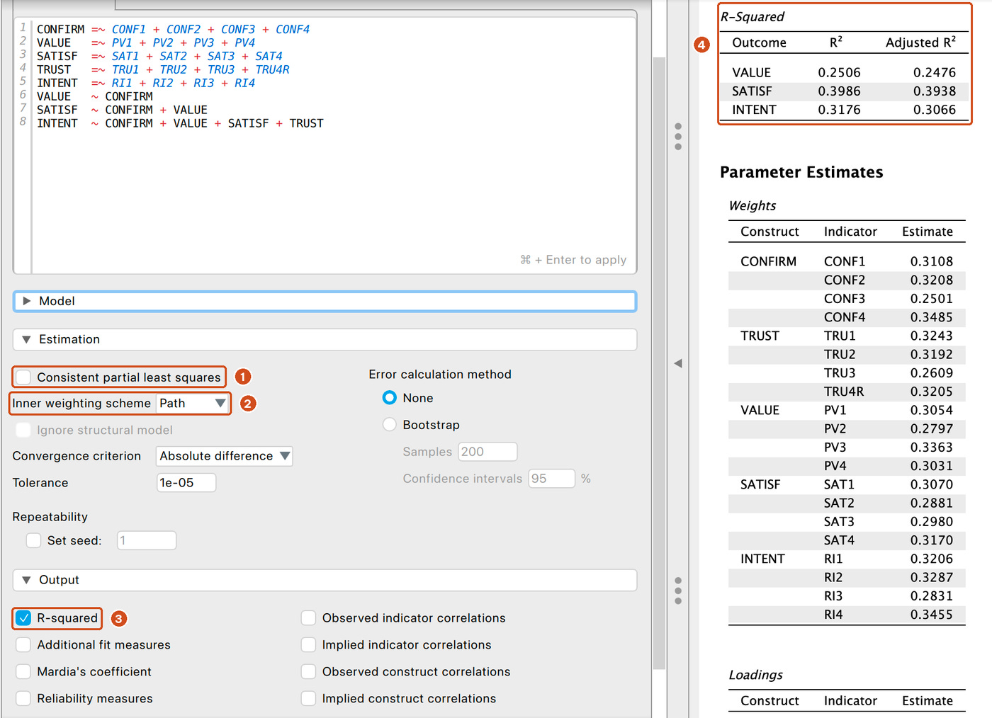
marketplace_x_sem_complete.savin JASP.Choose SEM > Partial Least Squares SEM (Figure 4).
Type the model syntax below in the model box and press Cmd + Enter to apply it (the box shows this hint).
Expand Estimation, untick Consistent partial least squares and keep Inner weighting scheme at Path (Figure 5).
Expand Output and tick R-squared.
CONFIRM =~ CONF1 + CONF2 + CONF3 + CONF4
VALUE   =~ PV1 + PV2 + PV3 + PV4
SATISF  =~ SAT1 + SAT2 + SAT3 + SAT4
TRUST   =~ TRU1 + TRU2 + TRU3 + TRU4R
INTENT  =~ RI1 + RI2 + RI3 + RI4
VALUE   ~ CONFIRM
SATISF  ~ CONFIRM + VALUE
INTENT  ~ CONFIRM + VALUE + SATISF + TRUST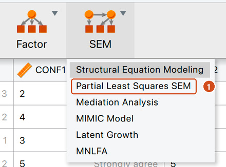
4. PLS-SEM or CB-SEM?
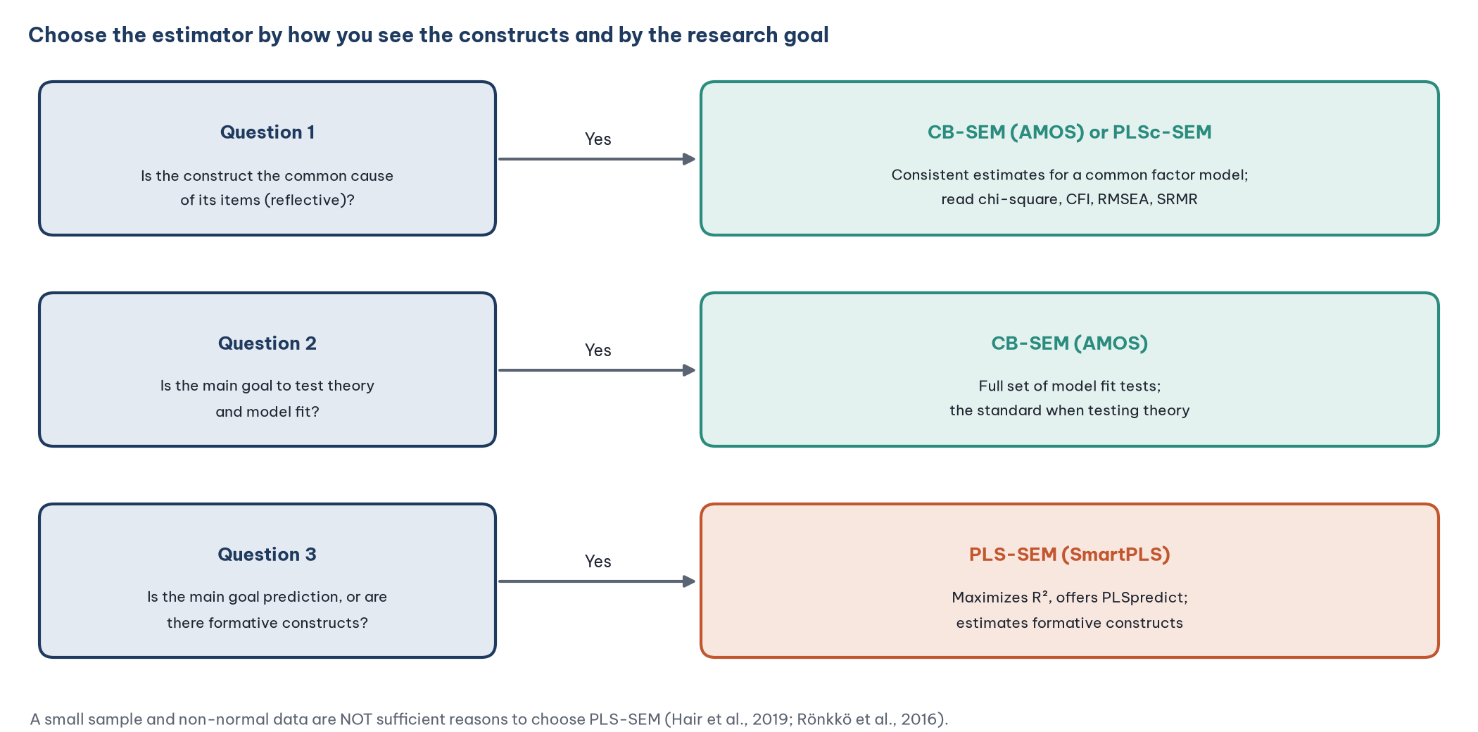
Two reasons that are not sufficient for choosing PLS-SEM, even though they are very common in theses:
"The sample is small." PLS-SEM runs with small samples, but that does not make the estimates more accurate; a small sample still gives low statistical power. Hair et al. (2019) themselves warn against using a small sample as the main reason, and Rönkkö et al. (2016) strongly criticize this argument. The sample size should be determined by a power analysis or the inverse square root method (Hair et al., 2022; Post 4, "How Large Should Your Sample Be? Formulas and Rules of Thumb for a Thesis").
"The data are not normal." CB-SEM has ways to deal with non-normal data: robust estimation (MLR) and the Bollen-Stine bootstrap (Post 22, "Confirmatory Factor Analysis (CFA) in JASP").
The debate about PLS-SEM continues. Its supporters stress its role in prediction and in composite models (Hair et al., 2019; Sarstedt et al., 2016). Its critics argue that PLS-SEM is often used for common factor constructs, where it gives biased estimates (Rönkkö et al., 2016). The safe approach in a thesis: state why you chose the method based on how you understand the constructs and on the research goal, not on sample size or distribution.
5. Software for PLS-SEM
This series follows the workflow in SmartPLS 4 and cross-checks it with JASP or R, so that readers without a SmartPLS license can still practice.
6. Roadmap of the SmartPLS series
Frequently asked questions
SmartPLS and AMOS give different results. Which should I report?
Report the results of the method you chose and explain why you chose it. Do not run both and then pick the "nicer" results. If you want to check robustness, report both, as in Section 3.
Do I need model fit with PLS-SEM?
PLS-SEM has no chi-square test like CB-SEM. SmartPLS reports SRMR; Hair et al. (2022) advise caution when using SRMR for PLS-SEM and recommend focusing on R², f², Q² and predictive power.
Should I choose PLS or PLSc in SmartPLS?
If your constructs are reflective and you care about the size of the coefficients, PLSc gives less biased estimates. If the goal is prediction or the constructs are composites, use PLS. State your choice in the methods section.
Can JASP replace SmartPLS?
For estimating the model, bootstrapping and PLSpredict, yes, because JASP uses the cSEM package. Some tools, such as drawing the model with the mouse or IPMA, are not available in the PLS-SEM module of JASP 0.99.0 (the module has only the sections Model, Estimation, Output and Prediction).
References
Dijkstra, T. K., & Henseler, J. (2015). Consistent partial least squares path modeling. MIS Quarterly, 39(2), 297–316. https://doi.org/10.25300/MISQ/2015/39.2.02
Hair, J. F., Hult, G. T. M., Ringle, C. M., & Sarstedt, M. (2022). A primer on partial least squares structural equation modeling (PLS-SEM) (3rd ed.). SAGE Publications.
Hair, J. F., Risher, J. J., Sarstedt, M., & Ringle, C. M. (2019). When to use and how to report the results of PLS-SEM. European Business Review, 31(1), 2–24. https://doi.org/10.1108/EBR-11-2018-0203
JASP Team. (2026). JASP (Version 0.99.0) [Computer software]. https://jasp-stats.org/
Rademaker, M. E., & Schuberth, F. (2026). cSEM: Composite-based structural equation modeling (R package version 0.7.1) [Computer software]. https://CRAN.R-project.org/package=cSEM
Ringle, C. M., Wende, S., & Becker, J.-M. (2026). SmartPLS 4 (Version 4.1.2.1) [Computer software]. SmartPLS GmbH. https://www.smartpls.com
Rönkkö, M., McIntosh, C. N., Antonakis, J., & Edwards, J. R. (2016). Partial least squares path modeling: Time for some serious second thoughts. Journal of Operations Management, 47–48, 9–27. https://doi.org/10.1016/j.jom.2016.05.002
Rosseel, Y. (2012). lavaan: An R package for structural equation modeling. Journal of Statistical Software, 48(2), 1–36. https://doi.org/10.18637/jss.v048.i02
Sarstedt, M., Hair, J. F., Ringle, C. M., Thiele, K. O., & Gudergan, S. P. (2016). Estimation issues with PLS and CBSEM: Where the bias lies! Journal of Business Research, 69(10), 3998–4010. https://doi.org/10.1016/j.jbusres.2016.06.007
Wold, H. (1982). Soft modeling: The basic design and some extensions. In K. G. Jöreskog & H. Wold (Eds.), Systems under indirect observation: Causality, structure, prediction (Part II, pp. 1–54). North-Holland.
Discussion about this post