Pearson Correlation in SPSS and PSPP: Run, Read and Report It
How to run a Pearson correlation in SPSS and PSPP, read r and its significance, handle outliers and report an APA-style correlation table


Key takeaways
Look at a scatter plot before you trust r: a curved relationship can give r close to 0, and one outlier can change r almost threefold.
Read the size of r and its confidence interval, not only the p-value; with N = 265, any r of about 0.12 is significant.
PSPP has no NONPAR CORR or PARTIAL CORR, but Spearman equals Pearson on ranks and a partial correlation equals the correlation of residuals.
Controlling for CONF and PV halves the SAT and RI correlation (0.435 to 0.221), a first hint that SAT is a mediator.
Correlation is not causation: a cross-sectional survey cannot show the direction of an effect.
You now have the five composite variables CONF, PV, SAT, TRU and RI (Post 10, "Recoding Variables and Computing Composite Scores in PSPP (SPSS)"), you have checked their reliability (Post 11, "Cronbach's Alpha in PSPP (SPSS)") and their factor structure (Post 12, "Exploratory Factor Analysis (EFA) in PSPP (SPSS)"). The next step in almost every thesis is a correlation analysis. The correlation matrix gives a first look at the relationships between the constructs. Are the variables related in the direction that theory predicts? Is any pair so highly correlated that the two are hard to tell apart? Is any variable almost unrelated to the outcome?
This post shows how to run a Pearson correlation in PSPP on the sample data set (marketplace_x_analysis.sav, 267 responses), how to read each number in the matrix and which interpretation mistakes are common. It also points out two commands that PSPP does not have (Spearman correlation and partial correlation) and shows equivalent ways to get them. Every result in this post is real output of the syntax file correlation.sps in the repository of this series (Free Software Foundation, 2026).
Sample data and scripts. The data file and the syntax file for this post are in the research-data-analysis repository on GitHub (folder
data/andscripts/). Download the whole repository with Code > Download ZIP.
About the figures. Figures 2 and 3 are real screenshots of PSPP 2.1.2 on macOS (Apple silicon Mac), taken in November 2026 with the data file
marketplace_x_analysis.sav(in thedata/folder of the repository). Figures 4, 5 and 7 are real output of the syntax filecorrelation.sps, run in PSPP 2.1.2 and exported from the Output Viewer (File > Export > PDF). Figure 1 (simulated data) and Figure 6 (the sample data) are drawn in Python.
1. What does the Pearson correlation coefficient measure?
The Pearson correlation coefficient, written r, measures the strength and direction of the linear relationship between two quantitative variables. Its value lies between -1 and +1:
Positive r: the two variables rise together. More satisfied customers have a higher repurchase intention.
Negative r: as one variable rises, the other falls. For example, the more a respondent worries that marketplace X does not keep its promises (the original item TRU4), the lower their trust.
The closer r is to -1 or +1, the closer the points lie to a straight line. r = 0 means no linear relationship, but it does not mean no relationship at all.
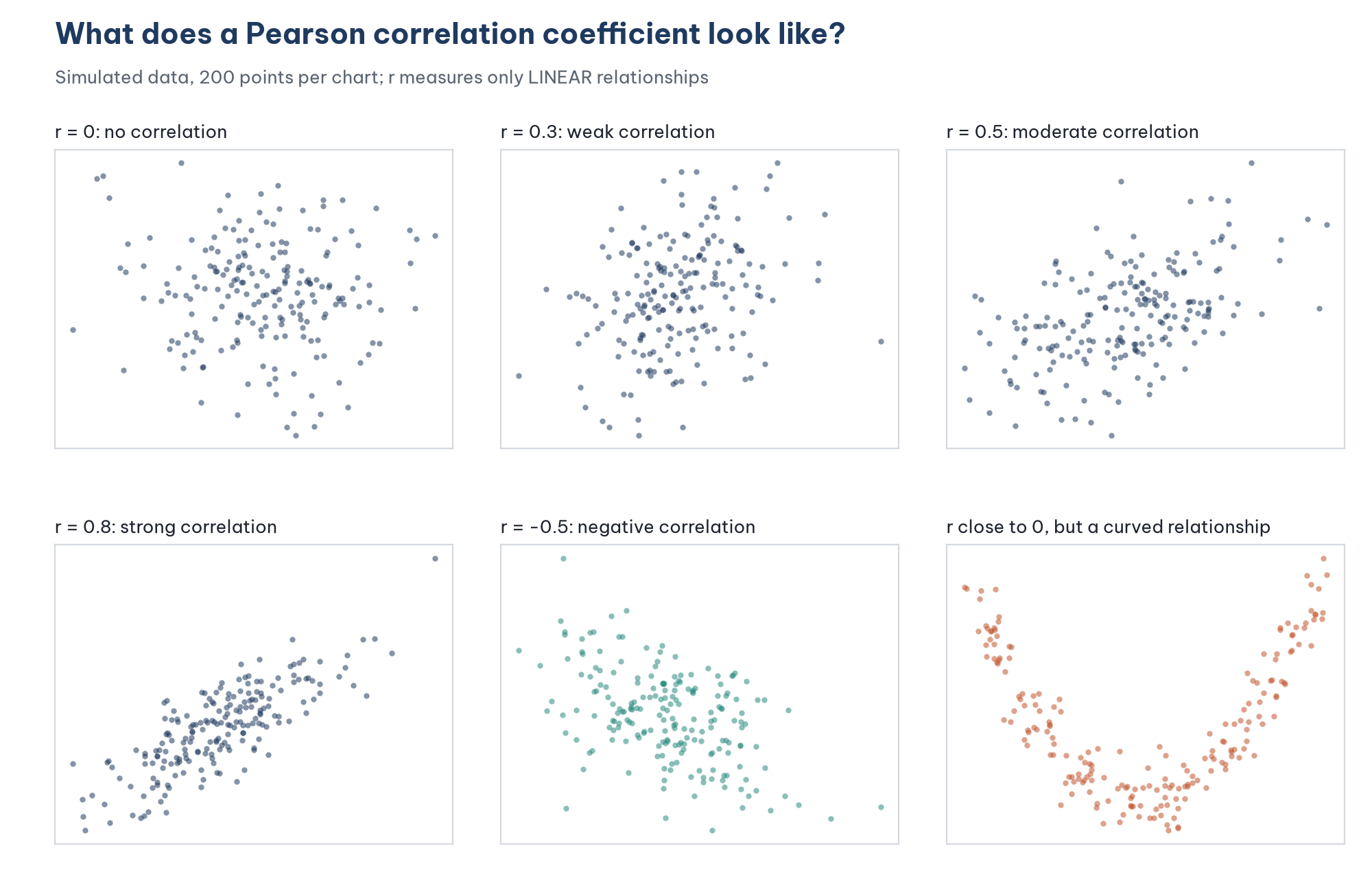
The last chart in Figure 1 is the reason you should always look at a scatter plot before you trust r. Anscombe (1973) made this point with four data sets that have the same correlation coefficient but completely different shapes.
The squared correlation, r*², is the *proportion of shared variance between the two variables. With r = 0.50, r*² = 0.25: 25% of the differences between respondents on one variable are "shared" with the other. Reading *r this way helps you avoid overstating it: a "moderate" correlation of 0.30 corresponds to only 9% shared variance.
Assumptions
According to Field (2024) and Tabachnick and Fidell (2019), a Pearson correlation is appropriate when:
Both variables are quantitative. A composite variable (the mean of 4 Likert items) meets this condition better than a single Likert item.
The relationship is linear. Check it with a scatter plot.
No outlier has a strong influence. A single extreme point can change r considerably (Section 5).
The distributions are close to normal, so that the significance test of r is accurate. With a sample of a few hundred, the test is fairly robust when the distributions are moderately skewed; when they are heavily skewed, use the Spearman correlation or the bootstrap (Bishara & Hittner, 2012).
2. Run a Pearson correlation in PSPP
With the menus
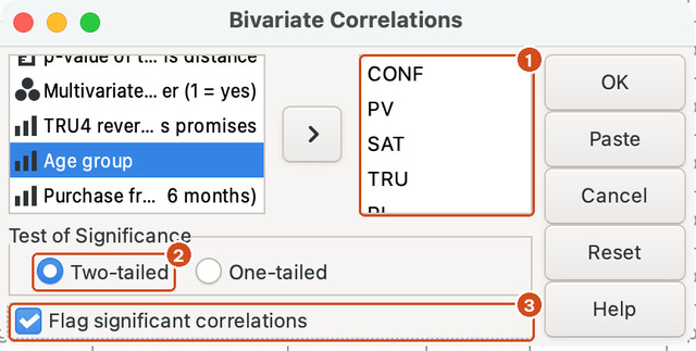
Choose Analyze > Bivariate Correlation (in SPSS: Analyze > Correlate > Bivariate). In the Bivariate Correlations dialog (Figure 2):
Move the five composite variables CONF, PV, SAT, TRU and RI into the box on the right (1). On the Mac the dialog is small, so the box shows only four names at a time; RI is the fifth, partly hidden at the bottom of the list.
Keep Two-tailed (2) under Test of Significance. Choose One-tailed only when your hypothesis stated the direction of the relationship before you collected the data, and you accept that you will ignore a relationship in the opposite direction.
Tick Flag significant correlations (3) so that PSPP marks the significant coefficients.
Click Paste to see the syntax (Figure 3). Note that in the syntax, NOSIG means flag the significant coefficients, not "not significant". The name comes from SPSS and is easy to misread.

With syntax
The PSPP dialog has no Options button to print descriptive statistics as SPSS does, but in syntax you can add /STATISTICS=DESCRIPTIVES:
CORRELATIONS /VARIABLES=CONF PV SAT TRU RI /PRINT=TWOTAIL NOSIG /STATISTICS=DESCRIPTIVES.3. Read the correlation matrix
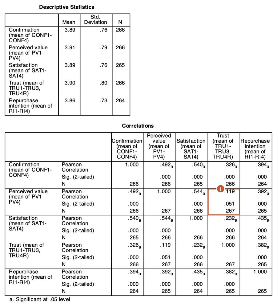
PSPP labels the rows and columns with the variable labels (for example "Satisfaction (mean of SAT1-SAT4)"), in the order CONF, PV, SAT, TRU, RI.
Three rows in each cell
Each cell of the matrix holds three numbers:
Pearson Correlation: the coefficient r.
Sig. (2-tailed): the p-value of the test of the hypothesis that r = 0 in the population.
N: the number of responses used to compute the coefficient.
The matrix is symmetric about the diagonal, so you only need to read the lower or the upper half. The diagonal is always 1, because every variable correlates perfectly with itself.
Size of the correlation
Cohen (1988) proposed three benchmarks: r = 0.10 is small, 0.30 is medium and 0.50 is large. Gignac and Szodorai (2016) reviewed more than 700 correlations from research on individual differences and found that benchmarks of 0.10, 0.20 and 0.30 reflect reality better. In other words, r = 0.30 is already a fairly large correlation in the social sciences.
Table 1 gives the results for the sample data, with 95% confidence intervals computed with the Fisher z transformation.
Read the results against the research model
A correlation matrix does not test causal hypotheses, but it shows whether the data are consistent with the model:
The outcome RI correlates positively and moderately with all four other variables (0.38 to 0.44). Its strongest correlation is with SAT (0.435), in line with the central role of Satisfaction in expectation-confirmation theory (ECM).
CONF and PV correlate strongly with SAT (0.54), in line with hypotheses H2 and H3 that Confirmation and Perceived value affect Satisfaction.
TRU correlates weakly with PV and SAT. In the model, Trust affects RI directly (H6), not through SAT. The low correlation between TRU and PV shows that the two constructs are fairly independent.
Significance depends on sample size
The PV – TRU pair has p = 0.051, just above the 0.05 threshold. With listwise deletion (/MISSING=LISTWISE, every coefficient uses the same 263 complete responses), the coefficient drops to 0.110 and p = 0.076. Two lessons follow from this example:
Significant versus not significant is not an absolute boundary. r = 0.119 with p = 0.051 and r = 0.125 with p = 0.04 are practically the same result. Report the confidence interval (-0.00 to 0.24) rather than only saying "not significant".
With a large sample, very small correlations are significant. With N = 265, any r of about 0.12 or more is significant at the 0.05 level. Statistical significance does not mean practical importance: r = 0.12 corresponds to only 1.4% shared variance.
By default, PSPP and SPSS use pairwise deletion: each coefficient uses every response that has both variables, so N differs from cell to cell (from 264 to 267). In your report, state how missing values were handled, or use listwise deletion so that every coefficient is based on the same sample.
4. Check linearity with a scatter plot
The GRAPH command draws a scatter plot (menu Graphs > Scatterplot):
GRAPH /SCATTERPLOT(BIVAR)=SAT WITH RI.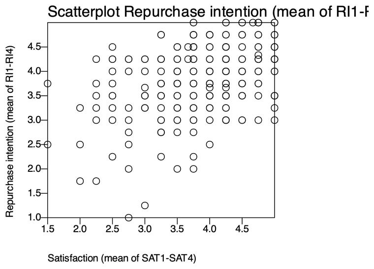
A composite of a 4-item scale takes only a limited number of values, so many responses fall on the same point. In the PSPP chart, the 264 responses show up as only 111 distinct points. The remedy is jittering: move each point by a very small random amount so that you can see the real density. Figure 6 redraws the chart this way in Python:
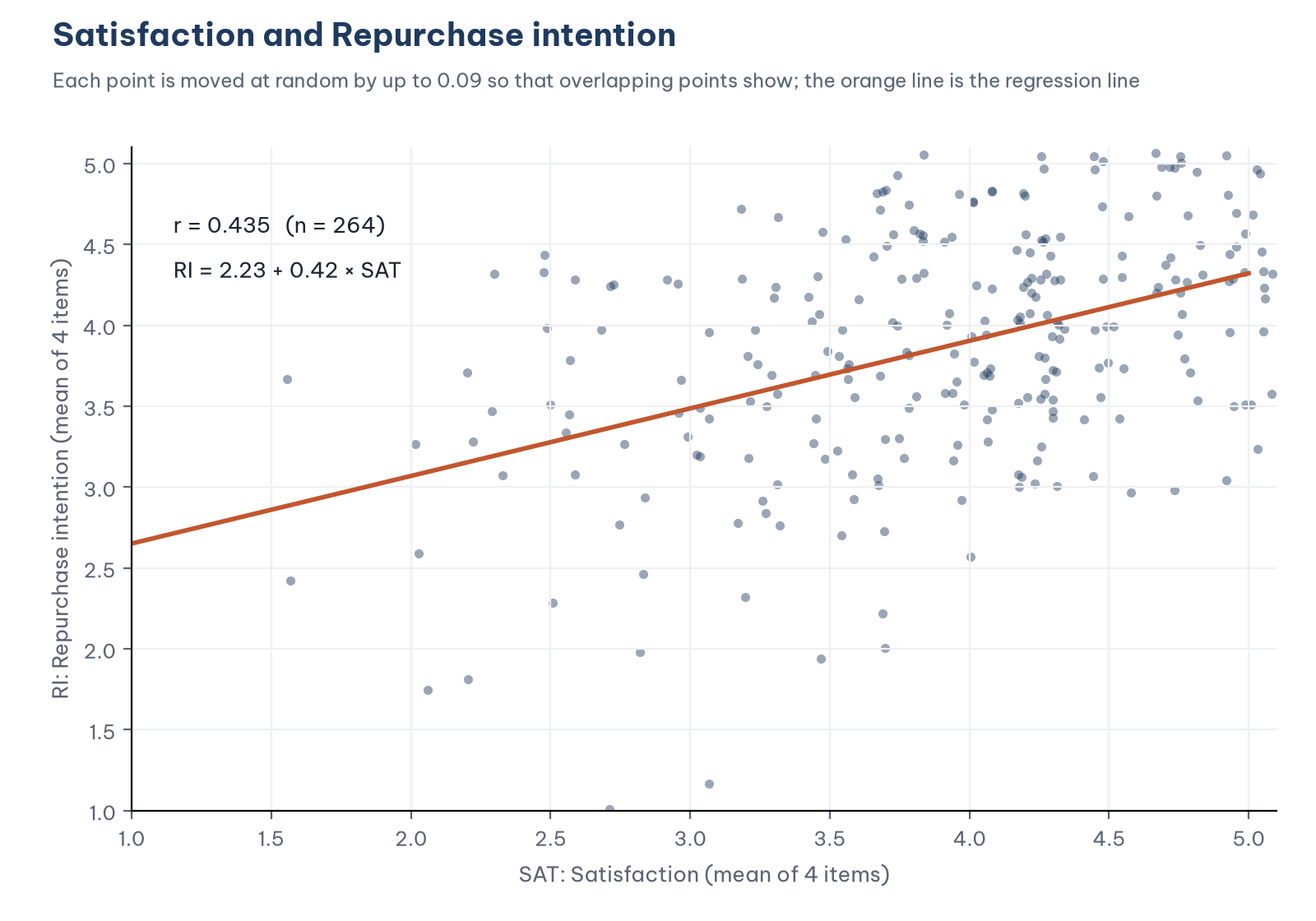
The relationship is linear: the points are spread around a rising straight line, with no curve and no separate cluster of points. The points are densest in the upper right corner, which matches the fact that most respondents are satisfied and intend to buy again.
5. The effect of outliers and the Spearman correlation
Post 8, "Data Cleaning in PSPP (SPSS)" kept response 99, with 95 purchases in 6 months. The scatter plot of the number of purchases (FREQ) against repurchase intention shows that this response lies far away from the rest:
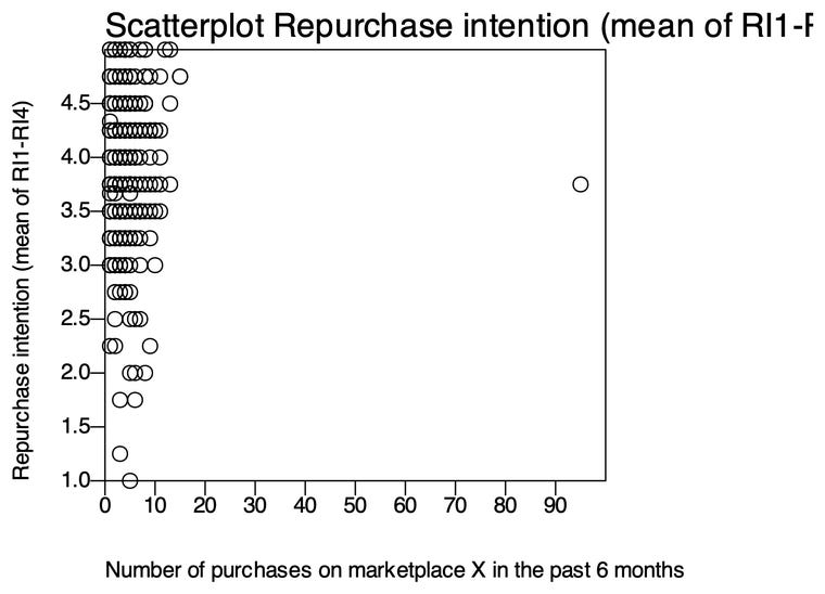
Table 2 shows three ways of computing the correlation between RI and FREQ.
A single response changes the Pearson coefficient almost threefold. Here the conclusion stays the same (no meaningful correlation), but with a smaller sample one outlier can turn a non-significant correlation into a significant one, or the other way round.
The Spearman rank correlation (written r*s or rho) computes the correlation on the *ranks of the data instead of the raw values. Response 99 is simply "the person who bought most"; whether they bought 95 or 16 times, the rank is the same. This is why Spearman is less affected by outliers, and why it suits ordinal variables or heavily skewed variables such as FREQ.
PSPP does not implement the NONPAR CORR command that SPSS uses for Spearman; the PSPP 2.1.2 manual lists it under "Not Implemented" (Free Software Foundation, 2026). Because Spearman is simply Pearson computed on ranks, the equivalent is to rank the variables with RANK and then run CORRELATIONS:
RANK VARIABLES=RI AGE FREQ (A) /RANK INTO R_RI R_AGE R_FREQ /TIES=MEAN.
CORRELATIONS /VARIABLES=R_RI R_AGE R_FREQ.
/TIES=MEAN gives tied values their average rank, which is how Spearman is defined. The result, 0.030, equals the value computed with the scipy library in Python. In SPSS, tick the Spearman box in the Bivariate Correlations dialog.
6. Partial correlation
SAT and RI correlate at 0.435. But both also correlate with CONF and PV. Part of the correlation between SAT and RI may exist only because people whose expectations were confirmed and who find marketplace X useful are both more satisfied and more willing to buy again. A partial correlation answers the question: how strongly are SAT and RI still correlated once the effect of CONF and PV is removed?
PSPP does not implement PARTIAL CORR either (it is also on the "Not Implemented" list of the manual). The equivalent follows from the definition of a partial correlation: take the residuals of SAT after regressing it on CONF and PV, take the residuals of RI after regressing it on CONF and PV and correlate the two sets of residuals:
DATASET NAME MAIN.
DATASET COPY PARTIALR.
DATASET ACTIVATE PARTIALR.
SELECT IF NMISS(SAT, RI, CONF, PV) = 0.
REGRESSION /VARIABLES=CONF PV /DEPENDENT=SAT /SAVE=RESID.
RENAME VARIABLES (RES1 = E_SAT).
REGRESSION /VARIABLES=CONF PV /DEPENDENT=RI /SAVE=RESID.
RENAME VARIABLES (RES1 = E_RI).
CORRELATIONS /VARIABLES=E_SAT E_RI.
The SELECT IF command runs on a copy of the data, so that both sets of residuals are computed on the same 263 responses without losing any responses from the main data set.
Result: the partial correlation between SAT and RI is 0.221 (p < .001), half of the simple correlation of 0.435. About half of the relationship between SAT and RI is explained by CONF and PV. The rest is the specific relationship between Satisfaction and Repurchase intention. This is a first hint of the mediating role of SAT, which will be tested formally in the regression and structural model posts.
A technical note: the CORRELATIONS command computes the p-value with n - 2 degrees of freedom, whereas a partial correlation controlling for two variables has n - 4. With 263 responses the difference is negligible. In SPSS, use Analyze > Correlate > Partial.
7. Correlation and the next steps of the analysis
The correlation matrix is also used for two preliminary checks:
Multicollinearity. The regression in Post 14, "Multiple Linear Regression in PSPP (SPSS)" uses CONF, PV, SAT and TRU as independent variables. If two independent variables correlate very highly (about 0.80 or more), the regression has difficulty separating the effect of each one. The largest correlation between the independent variables here is 0.544 (PV – SAT), which is no cause for concern. The formal check with the VIF is done in Post 15, "Checking Regression Assumptions in PSPP (SPSS)".
Discriminant validity. Two scales that measure different constructs should not correlate too highly. Kline (2016) treats a correlation of 0.85 or more between two latent variables as a sign that they are hard to distinguish. All correlations here are below 0.55. Discriminant validity is tested more rigorously with AVE and HTMT in the CB-SEM and SmartPLS parts of the series (Post 25, "Convergent and Discriminant Validity in JASP" and Post 35, "Discriminant Validity in SmartPLS 4").
Correlation is not causation. The fact that SAT correlates with RI does not prove that raising satisfaction will raise repurchase intention. The relationship could run the other way, or both could be caused by a third variable. A cross-sectional survey design such as this one cannot prove causation; theory is the basis for the direction of the effects in the model.
8. Present the correlation table in APA style
In theses and journal articles, the correlation table usually combines the descriptive statistics, the correlation matrix and Cronbach's alpha (American Psychological Association, 2020), as in Table 3.
Three APA conventions: show only the lower half of the matrix, number the columns instead of repeating the variable names and give the significance levels in a note under the table. PSPP marks significance at the 0.05 level with "a", whereas reported tables usually use one asterisk for p < .05 and two for p < .01.
Sample paragraph: "Table 4.x presents the descriptive statistics and Pearson correlations between the study variables. Repurchase intention correlated positively and moderately with Satisfaction (r = 0.44, 95% CI [0.33, 0.53]), Confirmation (r = 0.39), Perceived value (r = 0.39) and Trust (r = 0.38), all significant at p < .001. Satisfaction correlated strongly with Confirmation and Perceived value (r = 0.54). The correlation between Perceived value and Trust was small and not statistically significant (r = 0.12, p = .051). All correlations between the independent variables were below 0.60, suggesting a low risk of multicollinearity."
Five common mistakes
Running a correlation without looking at the scatter plot, and missing a curved relationship or an outlier.
Interpreting a correlation as a causal relationship, for example "satisfaction increases repurchase intention by 0.435".
Reporting only "significant" or "not significant" without the size of r and its confidence interval.
Using Pearson for heavily skewed variables or variables with outliers such as the number of purchases, instead of Spearman or a check without the outlier.
Choosing a one-tailed test after seeing the results, to turn p = 0.051 into p = 0.026.
Frequently asked questions
Should I run correlations for the individual items instead of the composite variables?
The correlation matrix of the items is used in EFA (Post 12). To describe the relationships between the constructs of the model, use the composite variables, because a composite measures a construct more reliably than any single item.
If a correlation is not significant, should I drop the variable from the regression model?
Not for this reason alone. The model is built from theory, and a variable with a small simple correlation can still have a unique effect once the other variables are controlled for (or the other way round). In the sample data, every independent variable correlates significantly with the outcome RI.
Can I use the Pearson correlation for single Likert items?
It is widely used, for example in EFA. However, for a 5-point Likert item, the Spearman correlation or the polychoric correlation reflects the ordinal nature of the data better. For composite variables made of several items, Pearson is a reasonable choice.
References
American Psychological Association. (2020). Publication manual of the American Psychological Association (7th ed.). https://doi.org/10.1037/0000165-000
Anscombe, F. J. (1973). Graphs in statistical analysis. The American Statistician, 27(1), 17–21. https://doi.org/10.1080/00031305.1973.10478966
Bishara, A. J., & Hittner, J. B. (2012). Testing the significance of a correlation with nonnormal data: Comparison of Pearson, Spearman, transformation, and resampling approaches. Psychological Methods, 17(3), 399–417. https://doi.org/10.1037/a0028087
Cohen, J. (1988). Statistical power analysis for the behavioral sciences (2nd ed.). Lawrence Erlbaum Associates.
Field, A. (2024). Discovering statistics using IBM SPSS Statistics (6th ed.). SAGE Publications.
Free Software Foundation. (2026). GNU PSPP (Version 2.1.2) [Computer software]. https://www.gnu.org/software/pspp/
Gignac, G. E., & Szodorai, E. T. (2016). Effect size guidelines for individual differences researchers. Personality and Individual Differences, 102, 74–78. https://doi.org/10.1016/j.paid.2016.06.069
Kline, R. B. (2016). Principles and practice of structural equation modeling (4th ed.). Guilford Press.
Tabachnick, B. G., & Fidell, L. S. (2019). Using multivariate statistics (7th ed.). Pearson.
Discussion about this post