Exploratory Factor Analysis (EFA) in SPSS and PSPP, Step by Step
How to run and read an EFA in SPSS and PSPP, from KMO and Bartlett’s test to the number of factors and the pattern matrix


Key takeaways
PSPP differs from SPSS in three places: it analyzes the covariance matrix by default, offers Promax only in syntax and has no KMO option in the dialogs.
Use principal axis factoring with Promax when constructs are expected to correlate; here factor correlations reach 0.62.
Decide the number of factors from several criteria: eigenvalues, the scree plot, PAF-based parallel analysis and theory all support 5 factors.
Read the pattern matrix, not the structure matrix; all 20 items load on their own factor (0.56 to 0.85) with no cross-loading of 0.30 or more.
Remove only one problem item at a time, then rerun the EFA, Cronbach's alpha and the composite scores.
Post 11, "Cronbach's Alpha in PSPP (SPSS)" showed that all five scales have good Cronbach's alpha values. But alpha only tells you that the items within one scale correlate with each other. It does not tell you whether item PV4, "Overall, marketplace X is useful for my shopping needs", really measures Perceived value, or whether respondents read it as something closer to Satisfaction. To find out whether the 20 questions split into the five groups of the model, you need an exploratory factor analysis (EFA).
This post shows how to run an EFA in PSPP on the 20 measurement items of the sample data set (marketplace_x_analysis.sav). It goes through six steps: checking the data, choosing the method, deciding the number of factors, reading the rotated matrix, handling problem items and reporting. It also points out three places where PSPP differs from SPSS; if you do not know them, you will get the wrong results.
Sample data and scripts. The data files and scripts for this post are in the research-data-analysis repository on GitHub (folder
data/andscripts/). Download the whole repository with Code > Download ZIP.
About the figures. Figures 3 to 6 are real screenshots of PSPP 2.1.2 on macOS (Apple silicon Mac), taken in November 2026 with the data file
marketplace_x_analysis.sav(in thedata/folder of the repository). Figures 2, 7, 8, 10, 11, 12a and 12b are real output of the syntax fileefa.spsin the repository, run in PSPP 2.1.2 and exported from the Output Viewer (File > Export > PDF). Tables that run over two pages of the export are joined, and the longest ones are laid out in two columns to save space; no value is changed. Figure 9 is drawn by the scriptefa_supplement.py(Free Software Foundation, 2026).
1. What EFA does and the six-step process
EFA looks for a small number of factors that explain most of the correlations among many questions. If the four items SAT1 to SAT4 correlate strongly with each other but weakly with the other items, EFA groups them into one factor. For a scale with a theoretical basis, as in this study, EFA checks whether the data support the proposed structure of five constructs. Testing that structure rigorously with a model is confirmatory factor analysis (CFA), covered in Post 22, "Confirmatory Factor Analysis (CFA) in JASP".
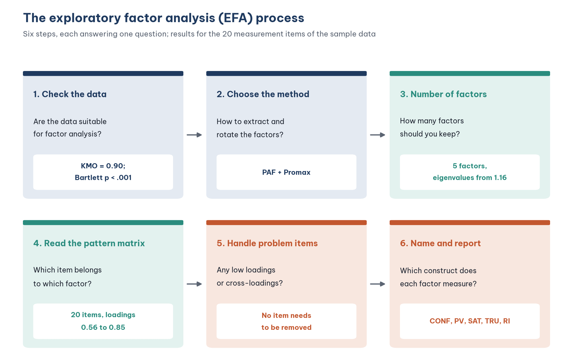
A common question is whether to run EFA separately for the independent and the dependent variables, or for all items together. Many theses run them separately. This post runs all 20 items together, for two reasons. First, the model has a mediator (Satisfaction is both an outcome of Confirmation and Perceived value and a cause of Repurchase intention), so it is hard to split the constructs into "independent" and "dependent". Second, a joint run checks whether the Repurchase intention items separate from the Satisfaction items, a first piece of evidence of discriminant validity.
2. Check the conditions before running EFA
Sample size
EFA uses listwise deletion: a response missing any of the 20 items is dropped. Of the 267 responses, EFA uses the 254 complete responses (Post 8, "Data Cleaning in PSPP (SPSS)"). Hair et al. (2019) suggest at least 5 observations per variable, preferably 10. Here the ratio is 254 / 20 = 12.7, which meets both levels and is above the minimum of 200 calculated for EFA in Post 4, "How Large Should Your Sample Be?".
KMO and Bartlett's test
These two statistics tell you whether the items correlate enough with each other for a factor analysis. They are in the first table of the output (Figure 2).

The KMO measure (Kaiser-Meyer-Olkin) compares the size of the ordinary correlations with the size of the partial correlations between items. A KMO close to 1 means that the correlation between any two items is largely explained by the other items, which is what you expect when there are common factors. Kaiser (1974) graded KMO as follows: 0.90 and above "marvelous", 0.80 and above "meritorious", 0.70 and above "middling", 0.60 and above "mediocre", 0.50 and above "miserable" and below 0.50 "unacceptable". The sample data have KMO = 0.90.
Bartlett's test of sphericity tests the hypothesis that the correlation matrix is an identity matrix, that is, that the items are not correlated at all. The result, p < .001, rejects this hypothesis. With a sample of a few hundred, Bartlett's test is almost always significant, so it is a necessary condition, not a sufficient one.
Besides the overall KMO, look at the MSA of each item (the item-level KMO). Items with an MSA below 0.50 should be considered for removal before running EFA (Hair et al., 2019). PSPP prints these values on the diagonal of the anti-image matrix (/PRINT=AIC), but that table is very large. The script efa_supplement.py in the repository computes all 20 values compactly: the lowest is TRU2 (0.84) and the highest is PV4 (0.93). The script also computes the determinant of the correlation matrix, 1.42 × 10⁻⁴, which is above the 10⁻⁵ threshold that Field (2024) uses as a warning of too much multicollinearity among the items.
3. Choose the extraction method and the rotation
Extraction method: PAF or PCA?
There are two common choices:
Principal components analysis (PCA) summarizes all of the variance of the items into components. PCA is the default in SPSS and PSPP.
Principal axis factoring (PAF) analyzes only the common variance shared by the items and leaves out the unique variance and measurement error of each item.
In theory, PCA is a data-reduction technique, while PAF is a true factor analysis: it looks for the latent constructs that cause the answers. Fabrigar et al. (1999) and Costello and Osborne (2005) both recommend PAF or maximum likelihood (ML) when the goal is to identify the structure of constructs. This post uses PAF. Section 7 compares it with PCA so that you can see the difference.
Rotation: Promax or Varimax?
The unrotated factor matrix is usually hard to read: most items load strongly on the first factor. Rotation redistributes the loadings so that each item loads strongly on a single factor. There are two families:
Orthogonal rotation, such as Varimax, assumes that the factors are uncorrelated.
Oblique rotation, such as Promax or Direct Oblimin, allows the factors to correlate.
In customer behavior research, constructs almost always correlate: more satisfied customers usually have a stronger intention to buy again. Assuming that they are uncorrelated is unrealistic. Tabachnick and Fidell (2019) suggest running an oblique rotation first and then looking at the factor correlation matrix. If correlations of 0.32 or more appear, an oblique rotation is appropriate. This post uses Promax, and Section 6 shows correlations between factors of up to 0.62.
4. Run EFA in PSPP
With the dialogs
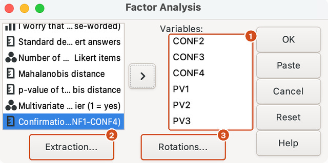
Choose Analyze > Factor Analysis. In the Factor Analysis dialog (Figure 3), move the 20 measurement items into the Variables box (1). Use TRU4R, the reverse-coded item, not TRU4, and do not include the attention-check item AC1 or the composite scores. On the Mac the dialog is small, so the Variables box shows only six items at a time (CONF1 is above CONF2 in the scrolled list in Figure 3). Then click Extraction (2) and Rotations (3) to set the options.
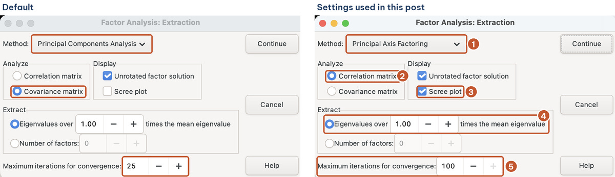
The Extraction dialog (Figure 4) has a trap: under Analyze, PSPP selects Covariance matrix by default, whereas SPSS uses the correlation matrix by default. Set it up as follows:
Method: choose Principal Axis Factoring.
Analyze: choose Correlation matrix. Analyzing the correlation matrix means standardizing every item before the analysis, and only then can the results be compared with guidelines and other studies.
Display: tick Scree plot (Unrotated factor solution is already ticked).
Extract: keep Eigenvalues over 1.00 times the mean eigenvalue. For a correlation matrix the mean eigenvalue is 1, so this criterion is the Kaiser criterion: keep factors with an eigenvalue greater than 1.
Maximum iterations for convergence: raise it from 25 to 100, so that PAF has enough iterations to converge.
The Rotation dialog (Figure 5) shows the second difference: the dialog offers only None, Varimax, Quartimax and Equimax (1). Promax is available only in syntax. Choose Varimax for now. The dialog has its own Maximum iterations box (2), set to 25. Click Continue, then click Paste in the main dialog to get the syntax and edit it.

Edit the syntax
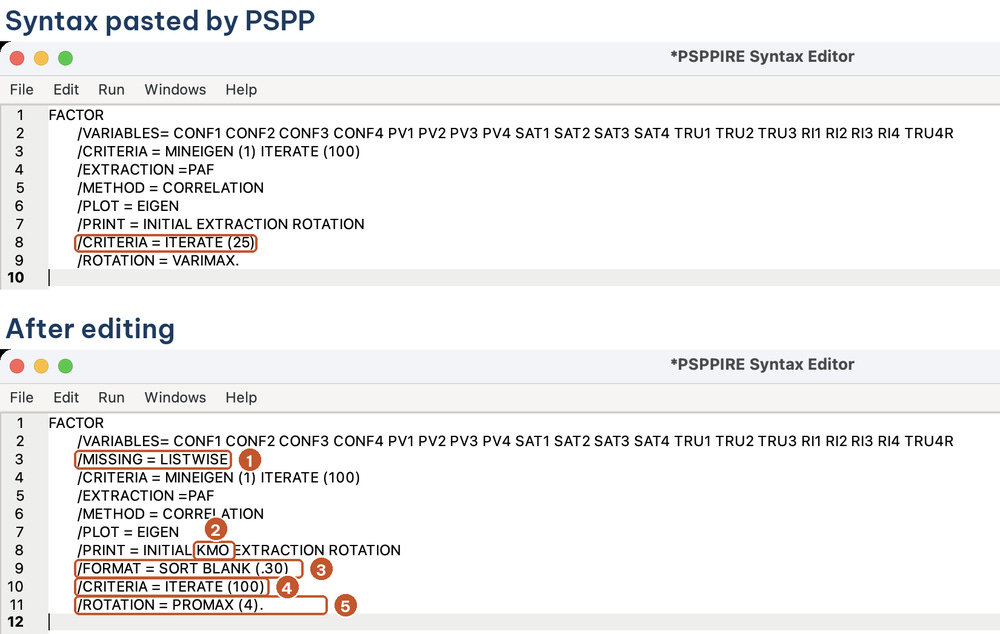
The syntax that PSPP pastes (Figure 6, top) needs five changes (Figure 6, bottom). This is also the third difference: the PSPP dialogs have no KMO option, so you have to add it by hand. Note the second /CRITERIA = ITERATE (25) line: it comes from the iteration box of the Rotation dialog; change it to 100 as well, so that both limits match the setting in the Extraction dialog.
The efa.sps file in the repository writes the same command more compactly:
FACTOR
  /VARIABLES=CONF1 CONF2 CONF3 CONF4 PV1 PV2 PV3 PV4 SAT1 SAT2 SAT3 SAT4 TRU1 TRU2 TRU3 TRU4R RI1 RI2 RI3 RI4
  /MISSING=LISTWISE
  /PRINT=INITIAL KMO EXTRACTION ROTATION
  /PLOT=EIGEN
  /FORMAT=SORT BLANK(.30)
  /CRITERIA=MINEIGEN(1) ITERATE(100)
  /EXTRACTION=PAF
  /ROTATION=PROMAX(4).
/FORMAT=SORT BLANK(.30) sorts the items by the factor on which they load most strongly and hides loadings below 0.30, which makes the matrix much easier to read. In SPSS, the matching options are under the Options button (Sorted by size, Suppress small coefficients), and KMO is under the Descriptives button. The 4 in PROMAX(4) is the kappa parameter, the SPSS default.
In the Output Viewer, PSPP lists the items by their variable labels (the wording of each question) rather than by their names, as you can see in Figures 7 to 12b. The tables in this post use the names (CONF1, PV4 and so on); the codebook in Post 6, "Defining and Coding Variables in PSPP (SPSS)" links each name to its wording.
5. Decide the number of factors
Eigenvalues and variance explained
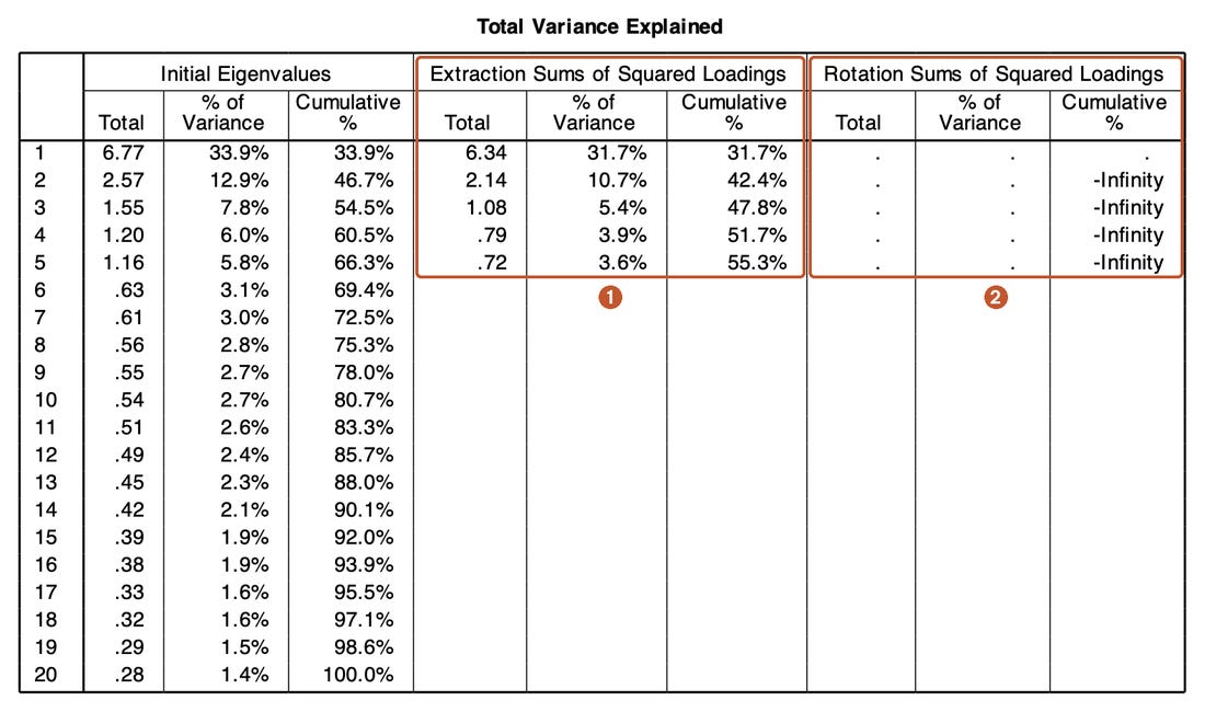
This table has three groups of columns:
Initial Eigenvalues: the eigenvalues of the original correlation matrix. The first five factors have eigenvalues of 6.77, 2.57, 1.55, 1.20 and 1.16. The sixth has only 0.63. By the Kaiser criterion, keep 5 factors, which explain 66.3% of the total variance.
Extraction Sums of Squared Loadings: the variance explained by the 5 factors after PAF extraction, 55.3%. This figure is always lower than with PCA, because PAF leaves out the unique variance of each item. Hair et al. (2019) consider factors that explain 60% of the variance or more satisfactory in the social sciences, and lower levels are common. Because PAF counts only the common variance, the variance explained by PAF is usually about 10 percentage points lower than with PCA, as here (55.3% against 66.3%).
Rotation Sums of Squared Loadings: with an oblique rotation the factors are correlated, so their variances overlap and cannot be added up into percentages. SPSS prints only the Total column in this case. PSPP prints dots and "-Infinity" instead. This is a display problem in PSPP, not a problem with your data; ignore this group of columns and report the variance explained from the second group.
The scree plot
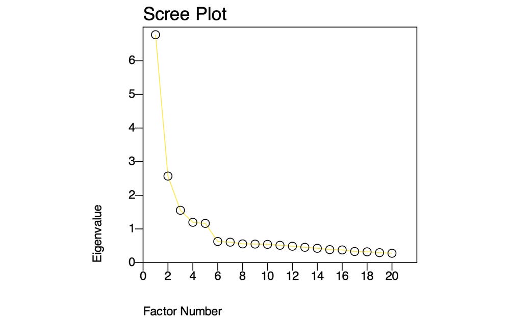
A scree plot shows the eigenvalues in order. The number of factors to keep is the number of points before the curve levels off. Here the curve breaks clearly between the fifth factor (1.16) and the sixth (0.63), which supports 5 factors.
Parallel analysis
The eigenvalue-greater-than-1 criterion tends to keep too many factors when there are many items (Costello & Osborne, 2005). Parallel analysis (Horn, 1965) is more reliable: it compares the eigenvalues of the real data with the eigenvalues of random data of the same size and keeps only the factors whose real eigenvalue is larger. PSPP and SPSS do not have this calculation built in. The script efa_supplement.py runs 1,000 simulations and gives a noteworthy result:
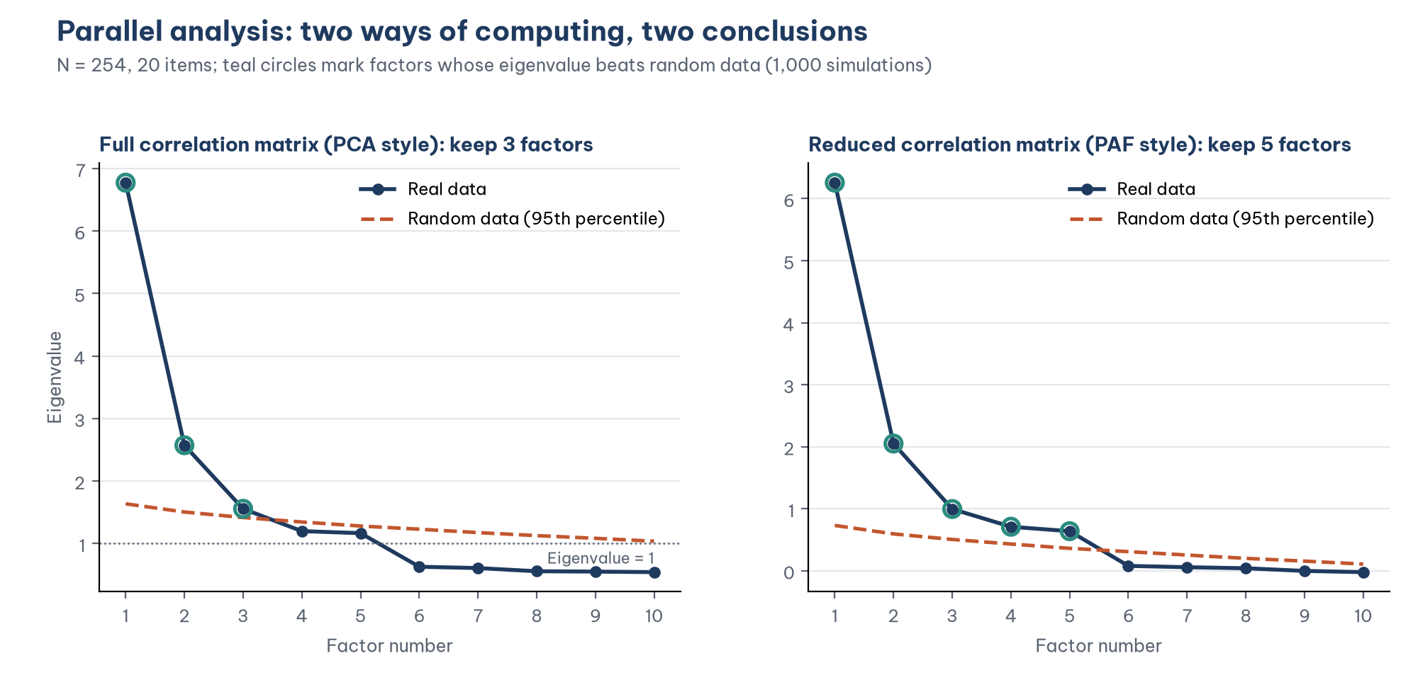
Table 1 shows the eigenvalues around the cut-off.
The two ways lead to two conclusions. Crawford et al. (2010) showed that PCA-based parallel analysis tends to keep too few factors when the factors are correlated, which is exactly the case here. To check, the syntax file runs an extra EFA with exactly 3 factors (/CRITERIA=FACTORS(3)). The result is in Figure 12a (Section 7): the 12 items of CONF, PV and SAT are merged into a single factor, whereas expectation-confirmation theory treats them as three different constructs with causal relationships between them.
Taking all the evidence together, the Kaiser criterion, the scree plot, PAF-based parallel analysis and theory all support 5 factors. This is how the decision should be made: do not rely on a single criterion, and when the criteria disagree, look at which solution makes theoretical sense.
6. Read the rotated matrix
With an oblique rotation, PSPP prints two matrices: the Pattern Matrix and the Structure Matrix. The pattern matrix shows the unique contribution of each factor to an item, after taking the correlations between factors into account. The structure matrix shows the simple correlations between items and factors, which are inflated by the correlations between factors. Interpret and report the pattern matrix (Tabachnick & Fidell, 2019).
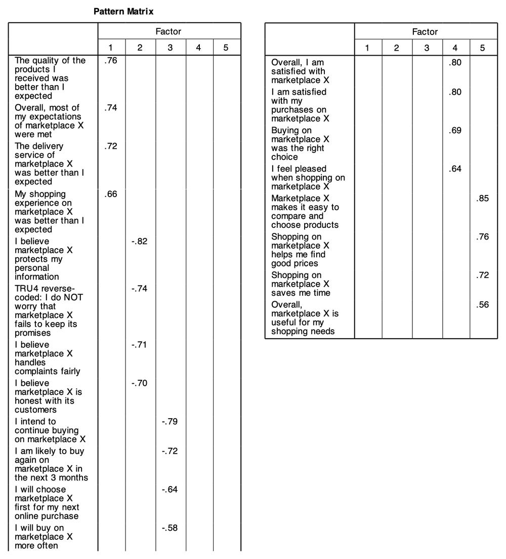
Judge the loadings
A factor loading shows how well an item reflects a factor. Two thresholds are commonly used:
Threshold based on sample size: Hair et al. (2019) state that with a sample of about 250, loadings of 0.35 or more are statistically significant.
Practical threshold: loadings of 0.50 or more are considered practically significant, and 0.70 or more indicates a well-defined structure (Hair et al., 2019).
Table 2 summarizes the five factors.
All 20 items load on the factor predicted by theory, with loadings of 0.56 or more. The weakest item is PV4 (0.56), which also had the lowest corrected item-total correlation in Post 11 and has the lowest communality (0.44). This is a notable agreement between the two analyses.
Why are some loadings negative?
All loadings of factors 2 and 3 are negative. This is not a sign that the items measure in the opposite direction. The direction of a factor is mathematically arbitrary: reversing the signs of all the loadings of a factor gives an equivalent solution. When all items of a factor share a negative sign, simply read the factor as "reversed" and flip the signs when you report. What should worry you is items within the same factor with different signs, as TRU4 would show if it were not reverse-coded: its sign would be opposite to that of TRU1 to TRU3.
Correlations between factors
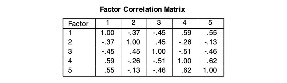
After flipping the signs of factor 2 (TRU) and factor 3 (RI), all correlations are positive, as theory expects (Table 3).
The largest correlation is between SAT and PV (0.62), followed by SAT and CONF (0.59), in line with hypotheses H2 and H3 that Confirmation and Perceived value affect Satisfaction. Many correlations exceed 0.32, which confirms that an oblique rotation is the right choice. None exceeds 0.70, the level often taken as a sign that two factors are hard to tell apart. Discriminant validity is tested more rigorously with AVE and HTMT in the CB-SEM and SmartPLS parts of the series (Post 25, "Convergent and Discriminant Validity in JASP" and Post 35, "Discriminant Validity in SmartPLS 4").
7. Compare with the alternatives
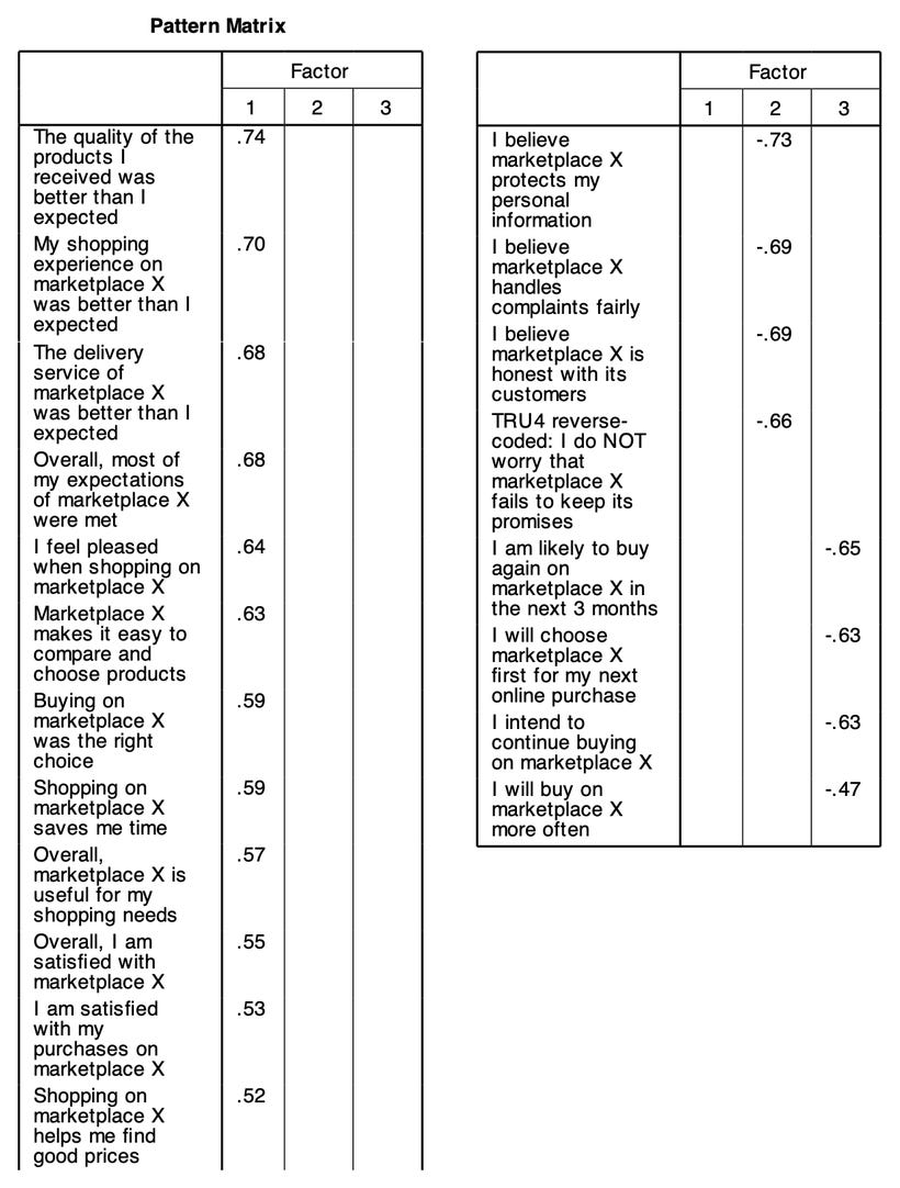
Figure 12a. Forcing 3 factors (PAF + Promax): the 12 items of CONF, PV and SAT merge into factor 1. The table is shown in two columns.
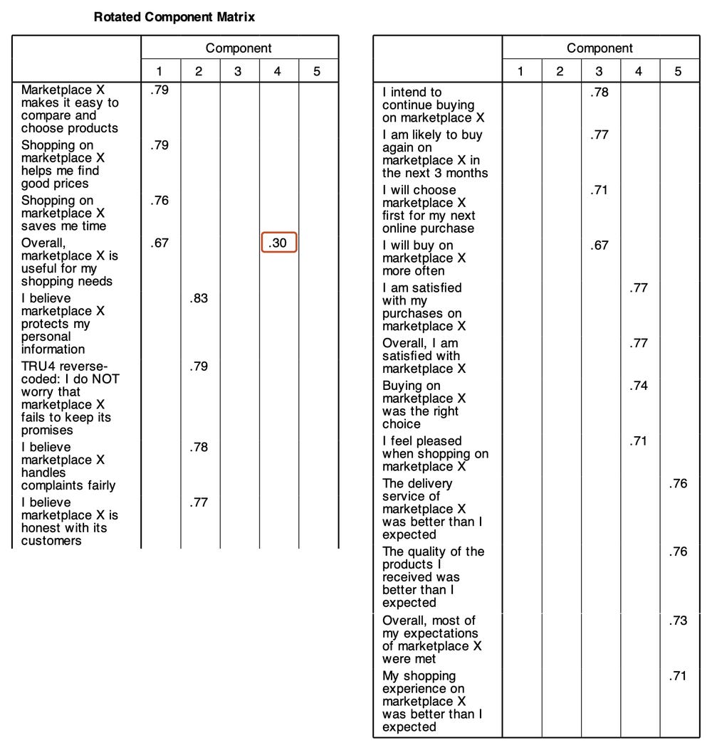
Figure 12b. PCA + Varimax gives the same five groups as PAF + Promax; PV4 cross-loads 0.30 on the Satisfaction component (frame). The table is shown in two columns.
The 3-factor solution (Figure 12a) merges Confirmation, Perceived value and Satisfaction into one factor, with loadings from 0.52 to 0.74. Statistically this solution is not "wrong", but it cannot separate three constructs that the model needs to keep apart to test the hypotheses.
PCA + Varimax (Figure 12b) is the default approach in many theses. With the sample data it gives the same five groups of items, higher loadings (0.67 to 0.83) and a higher total variance explained (66.3%). Higher loadings do not mean a better scale: PCA puts the unique variance of each item into the components as well. There is one notable difference: with Varimax, PV4 has a cross-loading of 0.30 on the Satisfaction component, because an orthogonal rotation forces the components to be uncorrelated while PV and SAT correlate at 0.62. With Promax this cross-loading disappears. When constructs are correlated, an orthogonal rotation can create "artificial" cross-loadings.
8. When should you remove an item?
The sample data give a clean result, but with real data you will often meet three situations:
Low loading: the item's highest loading is below 0.50 (or below 0.40 in exploratory research). The item does not reflect any factor well.
Cross-loading: the item loads 0.32 or more on two factors (Costello & Osborne, 2005), or its two loadings are about the same. The item does not distinguish between two constructs.
Item on the wrong factor: for example, a PV item that loads on the SAT factor. This can be a sign that the question is worded ambiguously.
The rule is the same as in Post 11: remove only one item at a time (the one with the most serious problem), then run the EFA again, because removing one item changes the whole solution. Consider the content of the item before removing it, make sure each factor keeps at least 3 items and record which items were removed and why. After removing items, run Cronbach's alpha again and recompute the composite scores.
9. Report the EFA results
The EFA table in a thesis usually lists the items grouped by factor, their pattern-matrix loadings and summary statistics at the bottom (Table 4).
Note: the eigenvalues in the last row follow the order of the factors before rotation, which does not necessarily match the order of the columns after rotation. Many authors report only the total variance explained to avoid this confusion.
Sample paragraph: "An exploratory factor analysis was run on the 20 measurement items (N = 254) using principal axis factoring with Promax rotation. The data were suitable for factor analysis (KMO = 0.90; Bartlett's test chi-square(190) = 2175.79, p < .001; item MSA from 0.84 to 0.93). The eigenvalue-greater-than-1 criterion, the scree plot and parallel analysis based on the reduced correlation matrix all supported 5 factors, explaining 55.3% of the variance. All 20 items loaded on their theoretical factor, with loadings from 0.56 to 0.85 and no cross-loadings of 0.30 or more. Correlations between factors ranged from 0.13 to 0.62."
Five common mistakes
Letting PSPP analyze the covariance matrix (the dialog default) instead of the correlation matrix.
Using a reverse-worded item that has not been reverse-coded, so that it loads negatively while the other items of the same factor load positively.
Using an orthogonal rotation when the constructs are correlated, which can create cross-loadings that are not real.
Relying only on the eigenvalue-greater-than-1 criterion to decide the number of factors, without checking the scree plot, parallel analysis and theory.
Reading the structure matrix instead of the pattern matrix with an oblique rotation, and seeing a series of "cross-loadings" caused by the correlations between factors.
Frequently asked questions
Some of my items load on a different factor from the one theory predicts. Do I have to remove them?
First, read the wording of the item again. It may be worded closer to the other construct, or respondents may have understood it differently from the questionnaire designer. If the wording shows that it really measures another construct, moving or removing the item must be clearly explained in the report. Do not quietly "move" an item to another factor just to get a nice result.
Should I run EFA before Cronbach's alpha?
Both orders are used. What matters is that the final results are consistent: Cronbach's alpha must be computed for the items of each factor as they stand after the EFA. If the EFA changes the composition of a scale, run alpha again.
Can EFA replace CFA?
No. EFA lets the data "speak for themselves" about how many factors there are and which item belongs to which factor; every item may load on every factor. CFA tests a specific structure set in advance, in which each item loads on only one factor, and it gives model fit indices. For a scale with a clear theoretical basis, as here, EFA is the first screening step, and CFA (Post 22) is the formal test.
References
Costello, A. B., & Osborne, J. W. (2005). Best practices in exploratory factor analysis: Four recommendations for getting the most from your analysis. Practical Assessment, Research, and Evaluation, 10(7). https://doi.org/10.7275/jyj1-4868
Crawford, A. V., Green, S. B., Levy, R., Lo, W.-J., Scott, L., Svetina, D., & Thompson, M. S. (2010). Evaluation of parallel analysis methods for determining the number of factors. Educational and Psychological Measurement, 70(6), 885–901. https://doi.org/10.1177/0013164410379332
Fabrigar, L. R., Wegener, D. T., MacCallum, R. C., & Strahan, E. J. (1999). Evaluating the use of exploratory factor analysis in psychological research. Psychological Methods, 4(3), 272–299. https://doi.org/10.1037/1082-989X.4.3.272
Field, A. (2024). Discovering statistics using IBM SPSS Statistics (6th ed.). SAGE Publications.
Free Software Foundation. (2026). GNU PSPP (Version 2.1.2) [Computer software]. https://www.gnu.org/software/pspp/
Hair, J. F., Black, W. C., Babin, B. J., & Anderson, R. E. (2019). Multivariate data analysis (8th ed.). Cengage Learning.
Horn, J. L. (1965). A rationale and test for the number of factors in factor analysis. Psychometrika, 30(2), 179–185. https://doi.org/10.1007/BF02289447
Kaiser, H. F. (1974). An index of factorial simplicity. Psychometrika, 39(1), 31–36. https://doi.org/10.1007/BF02291575
Tabachnick, B. G., & Fidell, L. S. (2019). Using multivariate statistics (7th ed.). Pearson.
Discussion about this post