Multiple Linear Regression in SPSS and PSPP: Output and Hypotheses
How to run multiple linear regression in SPSS and PSPP, read R-square, ANOVA and coefficients, test hypotheses and report the results


Key takeaways
A model with a mediator needs one regression equation for every variable with an arrow pointing into it; here three equations test six hypotheses.
Each coefficient B holds the other independent variables constant; compare the size of effects with Beta, not B.
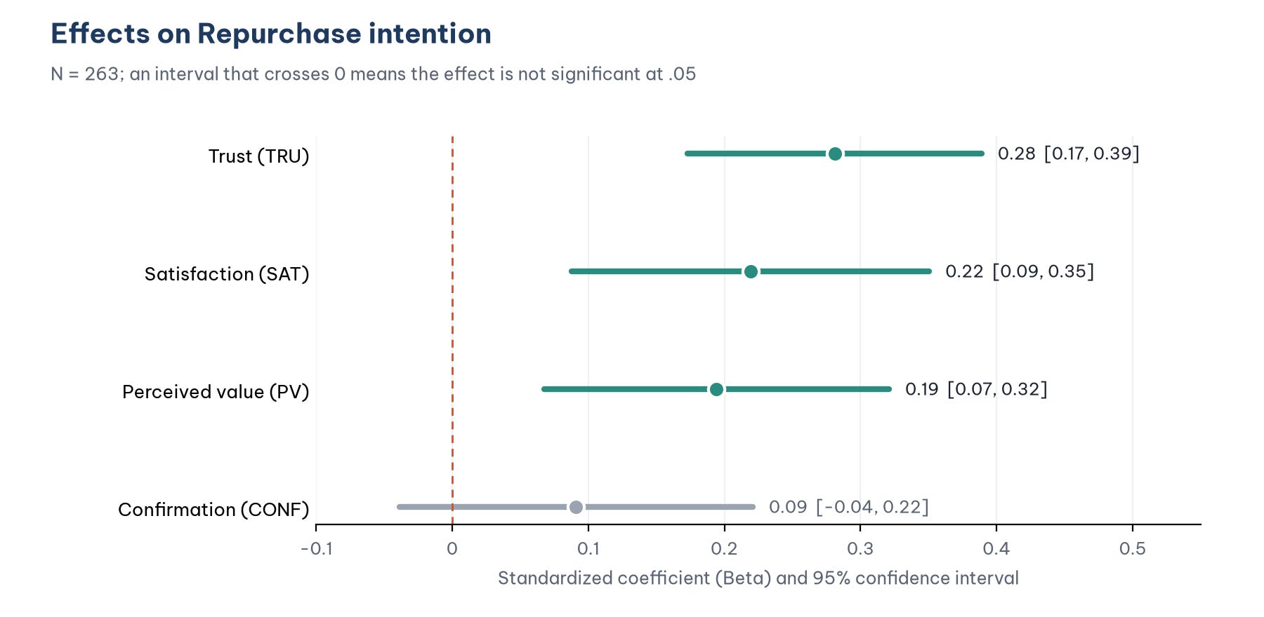
Model 2 explains 31.5% of repurchase intention (*f*² = 0.46, a large effect), and Trust has the largest Beta (0.28).
CONF is not significant once PV and SAT are in the equation, which fits the expectation-confirmation model rather than showing that CONF does not matter.
Compare *R*² in a hierarchical regression only on the same set of responses; adding SAT raises *R*² by 2.9%.
Post 13, "Pearson Correlation in PSPP (SPSS)" showed that Repurchase intention correlates with all four other constructs, but those four constructs also correlate with each other. The research question needs a sharper answer: when the factors are considered together, which ones really affect repurchase intention, and how strongly? That is the job of multiple linear regression.
This post uses regression to test the 6 hypotheses of the research model on the sample data set (marketplace_x_analysis.sav). It shows how to run the analysis in PSPP, how to read each output table, how to write the regression equation and how to report the results in a thesis. The assumptions of regression (distribution of the residuals, multicollinearity) are checked in detail in Post 15, "Checking Regression Assumptions in PSPP (SPSS)".
Sample data and scripts. The data files and scripts for this post are in the research-data-analysis repository on GitHub (folder
data/andscripts/). Download the whole repository with Code > Download ZIP.
About the figures. Figures 2 to 5 are real screenshots of PSPP 2.1.2 on macOS (Apple silicon Mac), taken in November 2026 with the data file
marketplace_x_analysis.sav(in thedata/folder of the repository). Figures 6 and 7 are real output of the syntax fileregression.spsin the repository, run in PSPP 2.1.2 and exported from the Output Viewer (File > Export > PDF); the Model 1 coefficients table runs over two pages of the export and is joined, with no value changed. Figures 1 and 8 are drawn in Python from the same data (Free Software Foundation, 2026).
1. The result first: the research model after regression
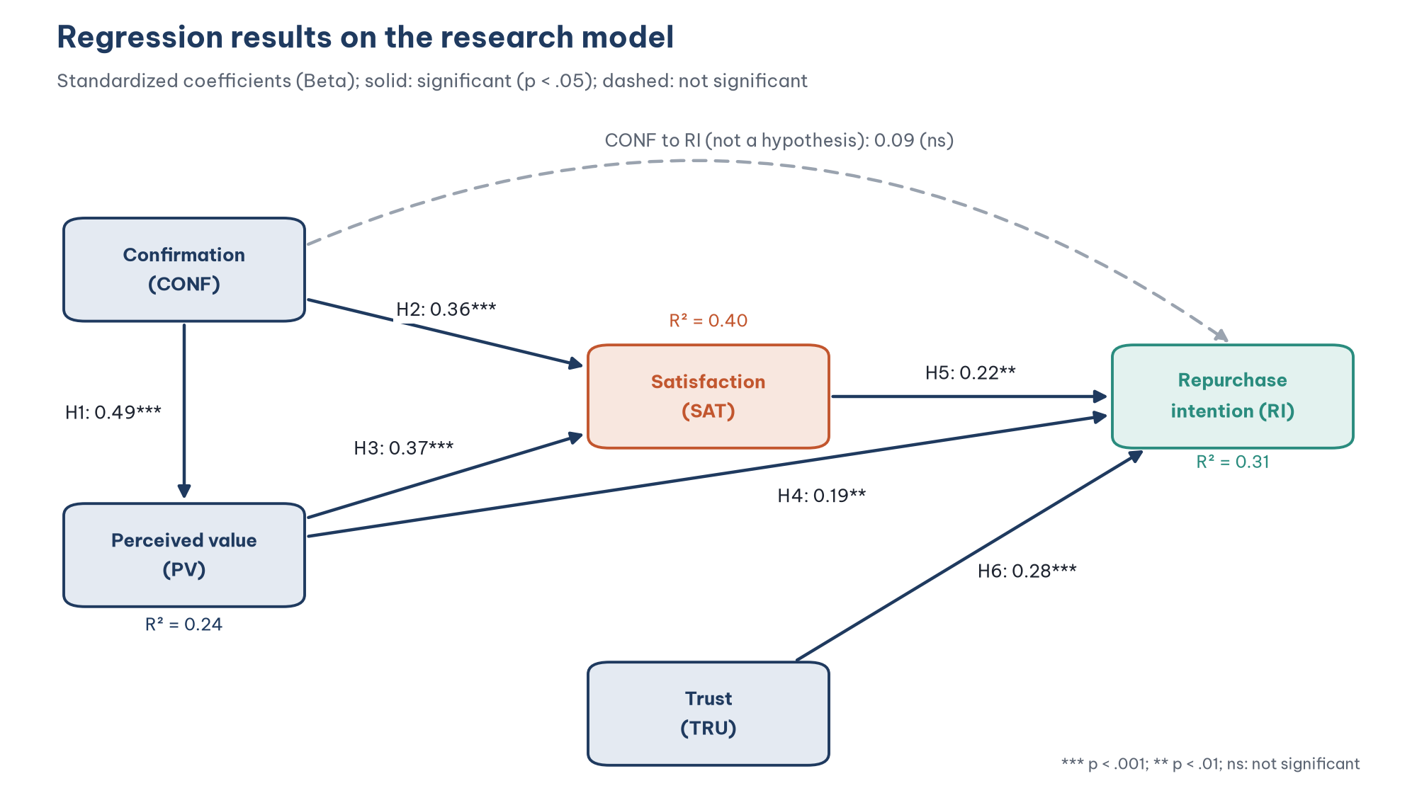
Figure 1 sums up the whole post. The sections below explain where each number comes from and how to read it.
2. What is multiple linear regression?
Multiple linear regression estimates one dependent variable Y from several independent variables *X*1, *X*2, ..., *X*k with the equation:
Y = B*0 + *B*1 × *X*1 + *B*2 × *X*2 + ... + *B*k × *X*k + *e
Each coefficient B tells you how much Y changes when the corresponding X increases by one unit, while the other independent variables are held constant. The phrase in bold is the most important difference between multiple regression and correlation. The correlation between CONF and RI is 0.39, but once PV, SAT and TRU are taken into account, the unique effect of CONF on RI may be much smaller (Cohen et al., 2003).
Three equations for the research model
The model has a mediator, SAT, so a single regression equation cannot test all the hypotheses. Every variable with an arrow pointing into it needs its own equation (Table 1).
In Model 2 there is no hypothesis of a direct effect of CONF on RI. In the expectation-confirmation model (ECM) of Bhattacherjee (2001), confirmation of expectations affects continuance intention through satisfaction and perceived usefulness. CONF is still included in Model 2 to check this: if the theory holds, CONF will have no significant direct effect once PV and SAT are in the equation.
Running separate regression equations is the traditional approach of path analysis. It gives no fit index for the model as a whole and does not account for measurement error. The CB-SEM and SmartPLS parts of the series estimate the whole model at once (Post 26, "Structural Equation Model (SEM) in JASP" and Post 37, "Evaluating the Structural Model in SmartPLS 4").
3. Run the regression in PSPP
With the menus
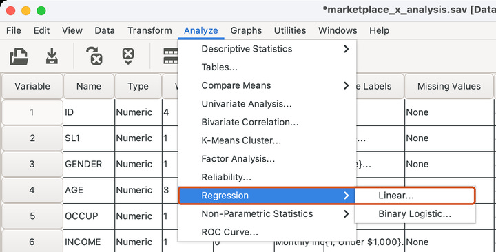
Choose Analyze > Regression > Linear (Figure 2). The Regression submenu of PSPP 2.1.2 has two commands, Linear and Binary Logistic.
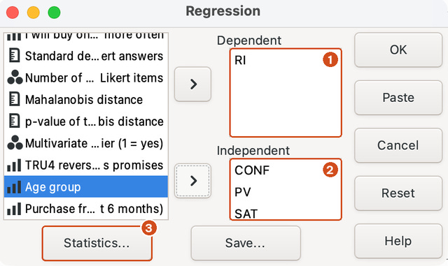
In the Regression dialog (Figure 3):
Move the dependent variable RI into the Dependent box (1).
Move the four independent variables CONF, PV, SAT and TRU into the Independent box (2). The box on macOS is small and shows only three rows; TRU is in the list below SAT (scroll the box to see it).
Click Statistics (3) to choose the output tables.
In the Statistics dialog (Figure 4), make sure Coeff, R and Anova are ticked, then also tick Conf. Interval (1) to get the 95% confidence interval of each coefficient B, and Tol (2) to get the Tolerance and VIF values used to check multicollinearity. On macOS the list shows only four rows at a time: Conf. Interval is near the top, and you have to scroll down to reach Bcov and Tol. Leave Bcov (the covariance matrix of the coefficients) unticked.

Click Continue, then Paste to get the syntax (Figure 5).

CI without a level; the syntax file below writes CI(95) to state the 95% level explicitly.With syntax
The file regression.sps runs all three equations:
REGRESSION /VARIABLES=CONF /DEPENDENT=PV /METHOD=ENTER
  /STATISTICS=COEFF CI(95) R ANOVA.
REGRESSION /VARIABLES=CONF PV /DEPENDENT=SAT /METHOD=ENTER
  /STATISTICS=COEFF CI(95) R ANOVA TOL.
REGRESSION /VARIABLES=CONF PV SAT TRU /DEPENDENT=RI /METHOD=ENTER
  /STATISTICS=COEFF CI(95) R ANOVA TOL.
Where PSPP differs from SPSS
Three limits of PSPP are worth knowing:
Only the Enter method (all variables entered at once). The Regression dialog has no method option, and in PSPP 2.0 the command
/METHOD=STEPWISEproduced an error. This is not a regrettable gap: stepwise methods (stepwise, forward, backward) choose the variables purely from the data, which gives unstable models and biased p-values (Smith, 2018; Whittingham et al., 2006). For research that tests hypotheses, Enter is the right method.No blocks of variables in one command (the dialog has no Next button) and, in PSPP 2.0, no
/STATISTICS=CHANGEto compute the change in *R*². Section 6 shows an equivalent way to do it.The Beta of the constant is printed as .00. SPSS leaves this cell empty. The constant has no standardized coefficient, so ignore this number.
4. Read the regression output
PSPP prints three tables for each equation. Figure 6 shows the output of Model 2.
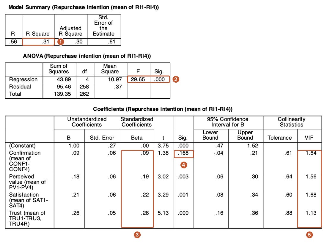
PSPP prints decimals without a leading zero (.31, .000), and it prints a p-value below .0005 as .000, which you should report as p < .001.
Model Summary: how much does the model explain?
R = 0.56 is the correlation between the observed RI values and the RI values predicted by the model.
R Square (R²) = 0.31 (1): the four independent variables explain 31.5% of the differences in repurchase intention between respondents. The remaining 68.5% is due to other factors outside the model and to error.
Adjusted R Square = 0.30 is *R*² adjusted for the number of independent variables and the sample size. *R*² always increases when you add a variable, even a meaningless one; adjusted *R*² does not. When you compare models with different numbers of variables, use adjusted *R*² (Field, 2024).
Std. Error of the Estimate = 0.61 is the standard error of the estimate: on average, the predicted values are about 0.61 points away from the observed values on the 1 to 5 scale.
Is R*² = 0.31 low or high? There is no general threshold, because human behavior is influenced by many factors outside the model. A more objective way to judge it is to convert it into the effect size f*² = *R*² / (1 − *R*²) = 0.46. Cohen (1988) considers *f*² = 0.02 small, 0.15 medium and 0.35 large, so Model 2 has a **large effect.
ANOVA: is the model significant?
The F test tests the hypothesis that all regression coefficients are zero, that is, that the model explains nothing. The result F(4, 258) = 29.65, p < .001 (2) rejects this hypothesis. The two numbers in brackets are the degrees of freedom: 4 independent variables, and 258 = 263 − 4 − 1, where 263 is the number of responses complete on all five variables.
A significant F test is a necessary condition. If F is not significant, do not interpret the individual coefficients.
Coefficients: how does each variable act?
This is the most important table. For each independent variable:
B (unstandardized coefficient): how many points RI increases when that variable increases by 1 point, with the other variables held constant. The B of TRU is 0.26: take two customers who are identical on CONF, PV and SAT, but one has a Trust score 1 point higher; that customer's expected repurchase intention is 0.26 points higher.
Std. Error: the standard error of B, which shows how precise the estimate is.
Beta (standardized coefficient) (3): the coefficient when every variable is standardized to a mean of 0 and a standard deviation of 1. Beta lets you compare the size of the effects of different variables. TRU has the largest Beta (0.28), followed by SAT (0.22) and PV (0.19).
t and Sig.: the test of the hypothesis that the coefficient is zero. CONF has t = 1.38, p = .168 (4), not significant at the 0.05 level.
95% Confidence Interval for B: the confidence interval of B. The interval for CONF runs from −0.04 to 0.21 and contains 0, which agrees with p > .05.
Tolerance and VIF (5): multicollinearity statistics. VIF ranges from 1.13 to 1.68 as printed (the exact largest value is 1.671), far below the warning thresholds (Hair et al., 2019); Post 15 discusses them in detail.
Model 1 and Model 0
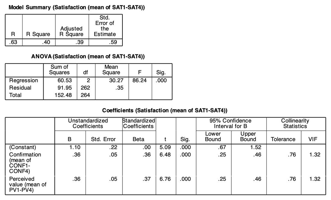
Model 1 explains 39.7% of the variance of Satisfaction (adjusted R*² = 0.39; *F(2, 262) = 86.24; p < .001; f*² = 0.66). Confirmation (*B = 0.36; Beta = 0.36; p < .001) and Perceived value (B = 0.36; Beta = 0.37; p < .001) have positive and almost equal effects.
Model 0 is a simple regression with one independent variable: CONF explains 24.2% of the variance of PV (B = 0.51; Beta = 0.49; t = 9.17; p < .001; N = 266). In a simple regression, Beta equals the Pearson correlation between the two variables (0.492 in Post 13).
5. Conclusions on the hypotheses
Table 2 brings the results of the three equations together.
Say "the data support the hypothesis" rather than "the hypothesis is proven". A cross-sectional study only shows that the data are consistent with the hypothesis; it does not prove a causal relationship.
CONF is not significant in Model 2: what does it mean?
Post 13 showed that CONF correlates 0.39 with RI. So why does CONF have almost no effect in Model 2? Because most of the influence of CONF on RI goes through SAT and PV: CONF increases PV (H1) and SAT (H2), and PV and SAT in turn increase RI. Once PV and SAT are in the equation, CONF has little unique information left to explain RI.
This is exactly what the ECM predicts. The result does not mean that CONF is unimportant: CONF matters because it is the starting point of the chain of effects. A formal test of this indirect effect (mediation analysis with bootstrapping) is covered in Post 28, "Mediation Analysis with JASP" and Post 40, "Mediation Analysis in SmartPLS 4".
6. Hierarchical regression: how much does SAT add?
Another question you might ask: once you know CONF, PV and TRU, how much better can you predict repurchase intention if you also know Satisfaction? Hierarchical regression answers this by entering the variables in blocks and comparing *R*².
SPSS does this in one command, with the Next button to create blocks and the R squared change option. PSPP has neither (the Regression dialog has no Next button, and PSPP 2.0 did not accept several blocks in one REGRESSION command), so the syntax file runs two models on the same set of complete responses (a copy of the data filtered to the 263 complete responses) and compares them:
DATASET NAME MAIN.
DATASET COPY COMPLETE.
DATASET ACTIVATE COMPLETE.
SELECT IF NMISS(CONF, PV, SAT, TRU, RI) = 0.
REGRESSION /VARIABLES=CONF PV TRU /DEPENDENT=RI /METHOD=ENTER /STATISTICS=R ANOVA.
REGRESSION /VARIABLES=CONF PV TRU SAT /DEPENDENT=RI /METHOD=ENTER /STATISTICS=R ANOVA.
You must use the same set of responses: on the full data, the model without SAT would use 264 responses and the model with SAT 263, and the two *R*² values would not be comparable.
PSPP prints *R*² to two decimals (.29 and .31); the three-decimal values above are the regression sums of squares divided by the total sum of squares in the ANOVA tables (39.88 / 139.35 and 43.89 / 139.35). The significance test of the *R*² change is computed from the two *R*² values:
F = (R*² change / number of variables added) / ((1 − *R*² of block 2) / (*N − k − 1)) = (0.029 / 1) / (0.685 / 258) = 10.83
where k = 4 is the number of variables in block 2 (the result 10.83 uses the unrounded R*² values). With degrees of freedom (1, 258), *p = .001. Satisfaction explains an extra 2.9% of the variance of repurchase intention, a small amount but statistically significant.
The R*² change when one variable is entered last is also called the *squared semipartial correlation (sr*²) of that variable: the share of variance explained *only by that variable. Table 4 gives it for the four variables.
The unique parts of the four variables add up to only 12.8%, while the model explains 31.5%. The remaining 18.7% is the shared part, explained jointly by independent variables that correlate with each other. This is why you should not read Beta as the "share" of each variable in *R*². Trust has the largest unique part because TRU correlates weakly with the other independent variables (Post 13).
Each sr*² can be computed from the Coefficients table: *sr*² = *t*² × (1 − *R*²) / (*N − k − 1). For TRU, 5.13² × 0.685 / 258 = 0.070.
7. The regression equation and prediction
From the B column of Model 2, the unstandardized regression equation is:
RI = 1.00 + 0.09 × CONF + 0.18 × PV + 0.21 × SAT + 0.26 × TRU
The standardized equation (with Beta, and no constant):
RI = 0.09 × CONF + 0.19 × PV + 0.22 × SAT + 0.28 × TRU
The unstandardized equation is used to predict on the original scale. For a customer who scores 4 points on all four variables, the expected repurchase intention is 1.00 + 0.09 × 4 + 0.18 × 4 + 0.21 × 4 + 0.26 × 4, about 3.93 with the unrounded coefficients (3.96 with the rounded ones shown). If Satisfaction rises to 5 points while the other variables stay the same, the expected repurchase intention rises by B = 0.21, to about 4.14. The standardized equation is used to compare the size of the effects of variables measured in different units.
This interpretation shows the practical meaning of the results: for Marketplace X, improving customer trust (protecting personal data, handling complaints fairly) has the largest unique effect on repurchase intention, alongside raising satisfaction.
8. Report the regression results
An APA-style table (American Psychological Association, 2020) usually combines the models in one table (Table 5).
Sample paragraph: "The regression results show that Confirmation (Beta = 0.36, p < .001) and Perceived value (Beta = 0.37, p < .001) have positive effects on Satisfaction, explaining 39.7% of its variance (F(2, 262) = 86.24, p < .001). Repurchase intention is positively affected by Trust (Beta = 0.28, p < .001), Satisfaction (Beta = 0.22, p = .001) and Perceived value (Beta = 0.19, p = .003); the model explains 31.5% of the variance (F(4, 258) = 29.65, p < .001). Confirmation has no significant direct effect on Repurchase intention (Beta = 0.09, p = .168), consistent with the argument of the ECM that the effect of confirmation on continuance intention runs through satisfaction and perceived usefulness. The data therefore support hypotheses H1 to H6."
Five common mistakes
Interpreting a coefficient B without the condition "the other variables held constant".
Comparing the size of effects with B instead of Beta when the variables are measured in different units.
Concluding that "CONF does not influence RI" just because the coefficient of CONF is not significant in a model with a mediator.
Using the stepwise method in research that tests hypotheses, letting the data decide which variables enter the model.
Comparing the R² of two models run on different sets of responses in a hierarchical regression.
Frequently asked questions
Is an R² of only 0.31 a sign of a poor model?
No. Repurchase intention depends on many factors outside the model, such as prices, promotions on competing marketplaces and personal habits. The goal of the study is to test the effects of specific variables, not to predict repurchase intention precisely. The effect size *f*² = 0.46 shows that the model has large practical significance.
Should I remove CONF from Model 2 and run it again?
It depends on your goal. If you only test hypotheses H4 to H6, you can drop CONF. Keeping CONF in the model still has value, though: it shows that the data are consistent with the ECM assumption of no direct effect. Report the model you chose and the reason for your choice.
Can a Beta coefficient be larger than 1?
Yes, when the independent variables correlate very strongly with each other, but that is usually a sign of serious multicollinearity. In the sample data the VIF values are low and every Beta is below 0.40. Post 15 shows how to check multicollinearity and the other assumptions of regression.
References
American Psychological Association. (2020). Publication manual of the American Psychological Association (7th ed.). https://doi.org/10.1037/0000165-000
Bhattacherjee, A. (2001). Understanding information systems continuance: An expectation-confirmation model. MIS Quarterly, 25(3), 351–370. https://doi.org/10.2307/3250921
Cohen, J. (1988). Statistical power analysis for the behavioral sciences (2nd ed.). Lawrence Erlbaum Associates.
Cohen, J., Cohen, P., West, S. G., & Aiken, L. S. (2003). Applied multiple regression/correlation analysis for the behavioral sciences (3rd ed.). Lawrence Erlbaum Associates.
Field, A. (2024). Discovering statistics using IBM SPSS Statistics (6th ed.). SAGE Publications.
Free Software Foundation. (2026). GNU PSPP (Version 2.1.2) [Computer software]. https://www.gnu.org/software/pspp/
Hair, J. F., Black, W. C., Babin, B. J., & Anderson, R. E. (2019). Multivariate data analysis (8th ed.). Cengage Learning.
Smith, G. (2018). Step away from stepwise. Journal of Big Data, 5, Article 32. https://doi.org/10.1186/s40537-018-0143-6
Whittingham, M. J., Stephens, P. A., Bradbury, R. B., & Freckleton, R. P. (2006). Why do we still use stepwise modelling in ecology and behaviour? Journal of Animal Ecology, 75(5), 1182–1189. https://doi.org/10.1111/j.1365-2656.2006.01141.x
Discussion about this post