Data Cleaning in SPSS and PSPP: Missing Values and Outliers
Seven steps to clean survey data in SPSS and PSPP, from invalid responses and entry errors to missing values and outliers, with syntax


Key takeaways
Remove invalid responses first (failed screening question, failed attention check, straight-lining); in the sample data this removed 33 of 300 responses.
Fix impossible values before you look for outliers. If the original questionnaire cannot be checked, set the cell to missing instead of guessing.
Measure how much is missing and check whether it is random; here only 0.39% of the scale cells were blank, and mean substitution is not recommended.
Only impossible values are errors. A genuine outlier, such as 95 purchases in 6 months, is kept, examined and reported.
Never overwrite the raw file: save a new clean file and keep a cleaning log for the methods section.
Survey data that has just been imported is almost never ready for analysis. Someone who has never bought anything still answers the whole questionnaire, someone else picks "Agree" for every item in a few seconds and a cell contains 55 instead of 5. If you feed these responses straight into Cronbach's alpha or a regression, the results can be wrong without the software giving any warning.
This post walks through a 7-step data cleaning process on the sample data set of 300 responses about repurchase intention on Marketplace X. The data set has the usual errors built in. Every number and result table in the post comes from a real run of the syntax file data_cleaning.sps from the GitHub repository of this series, in PSPP 2.1.2 on macOS (Free Software Foundation, 2026). The commands and menus are the same in SPSS.
Sample data and scripts. The data files and scripts for this post are in the research-data-analysis repository on GitHub (folder
data/andscripts/). Download the whole repository with Code > Download ZIP.
About the figures. Figures 2, 3, 4, 6 and 7 are cropped from the PSPP 2.1.2 Output Viewer after running
data_cleaning.spsonmarketplace_x_raw.sav(both in the repository), exported with File > Export > PDF. The comments in the syntax file number the blocks 1 to 8 because flagging and removing invalid responses are two separate blocks; the post groups them into one step.
1. Overview of the data cleaning process
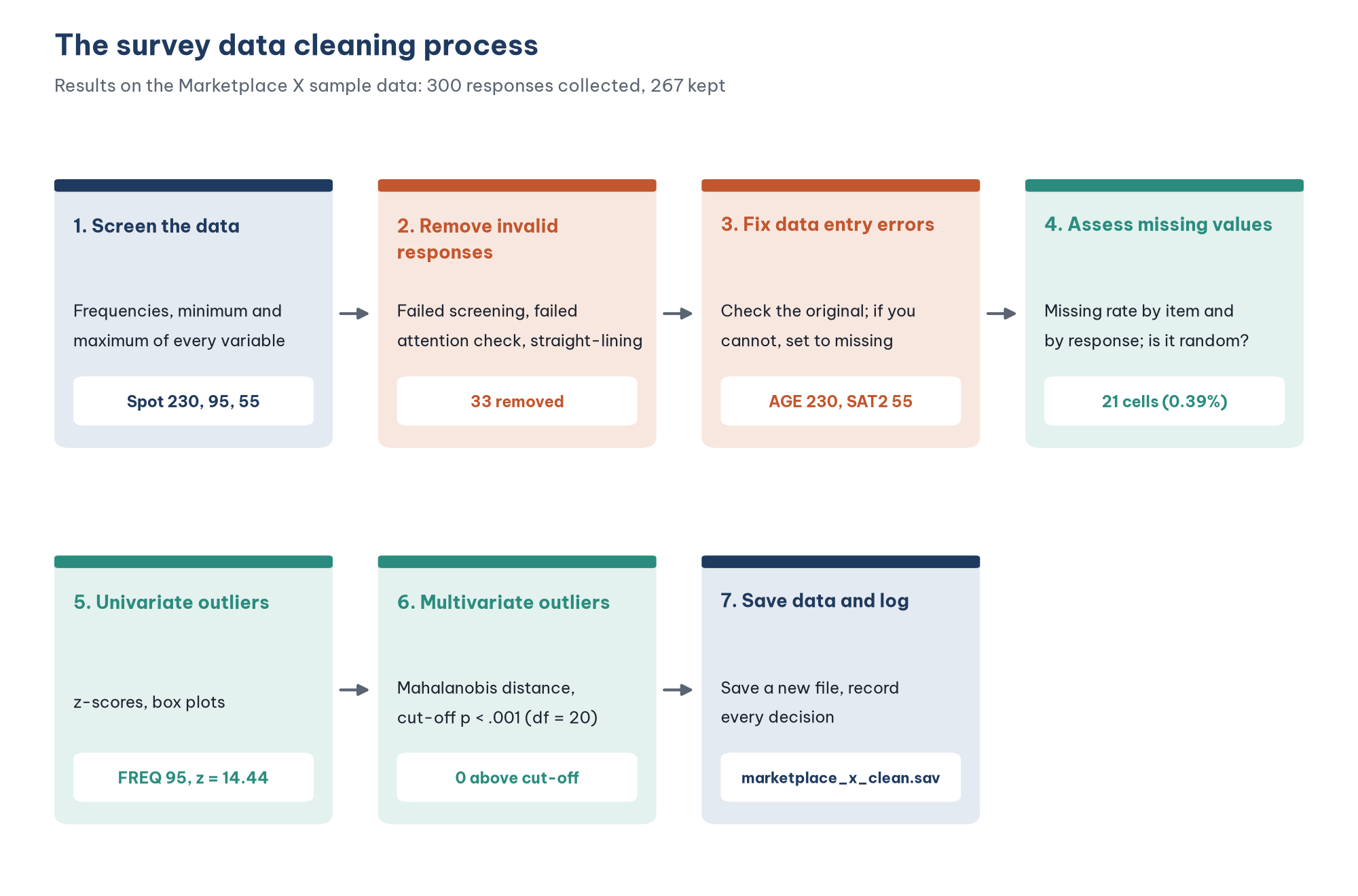
The order of the steps matters. Remove invalid responses first, before you assess missing values and outliers, because these responses distort the means, standard deviations and the covariance matrix that the later steps rely on. Fix data entry errors before you look for outliers, because a value of 55 on a 1 to 5 scale is an error to correct, not an unusual observation to think about.
One rule applies to the whole process: never overwrite the original file. The syntax file reads marketplace_x_raw.sav and saves the result as a new file, marketplace_x_clean.sav. Every decision is written in the syntax, so someone else (or you, three months later) can check it and run it again.
2. Step 1: Screen the data
The first job is to look at the range of values of every variable. The DESCRIPTIVES command (menu Analyze > Descriptive Statistics > Descriptives) gives the minimum, maximum, mean and standard deviation:
DESCRIPTIVES AGE FREQ CONF1 TO RI4 /STATISTICS=MEAN STDDEV MIN MAX.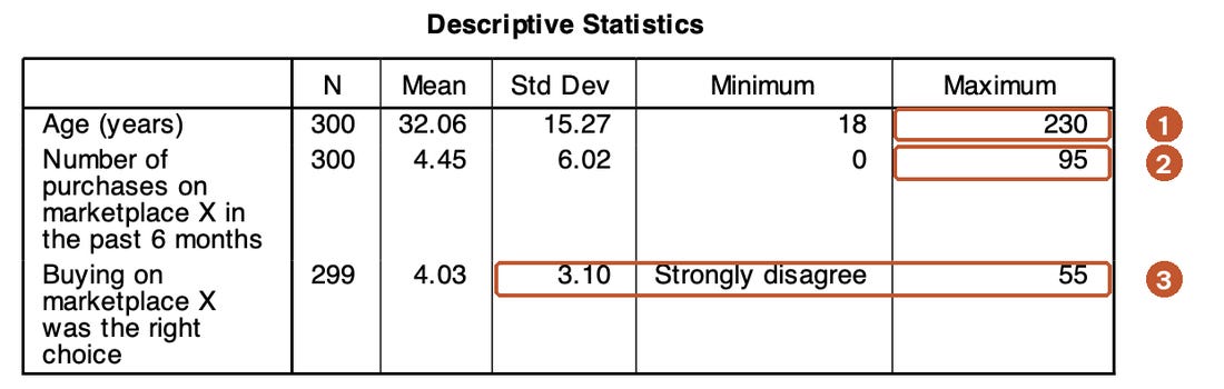
PSPP labels the rows with the variable labels, so SAT2 appears as "Buying on marketplace X was the right choice". Three warning signs stand out at once:
The largest age is 230. Nobody is 230 years old, so this is certainly a data entry error (most likely 23 with an extra 0).
The largest number of purchases is 95 in 6 months, while the mean is only 4.45. This value is unusual but possible: about 3 to 4 purchases a week. It is an outlier to examine in Step 5, not yet an error.
Item SAT2 has the value 55 on a 1 to 5 scale. This single wrong cell raises the standard deviation of SAT2 to 3.10, while the other scale items are between 0.90 and 1.01.
Also run FREQUENCIES for the control items (the screening question SL1 and the attention check AC1):
FREQUENCIES SL1 AC1 /STATISTICS=NONE.The frequency tables show that 14 respondents answered "No" to SL1 and 19 did not choose 2 ("Disagree") on AC1, "To check your attention, please select 2 for this item" (281 of 300 did).
A small tip: when Likert items have value labels, PSPP shows the Minimum and Maximum as labels ("Strongly disagree", "Strongly agree") instead of numbers. A value without a label, such as 55, is shown as a number, which makes it even easier to spot.
3. Step 2: Remove invalid responses
An invalid response is one that should not be in the sample, even if its answers look complete. There are three common types.
Responses that fail the screening question. The study is about customers who have bought on Marketplace X in the past 6 months, so the 14 respondents who answered "No" to SL1 are not part of the study population. Their opinions about "satisfaction with my purchases" are not based on real experience.
Responses that fail the attention check. An attention check (instructed response item) asks the respondent to choose a specific level. Meade and Craig (2012) recommend including such items in online surveys to detect careless respondents. Someone who does not follow such a clear instruction probably did not read the other items carefully either.
Responses with the same answer for every item (straight-lining). Curran (2016) calls this a long-string response pattern: the respondent picks the same level for a long run of consecutive items. The simplest way to detect it is to compute the standard deviation of the Likert items within one response. A standard deviation of 0 means every item has the same answer:
COMPUTE RESP_SD = SD(CONF1 TO SAT2, SAT3 TO RI4).The variable list skips AC1, because that item sits between SAT2 and SAT3 in the questionnaire. In the sample data, 8 responses have a standard deviation of 0:
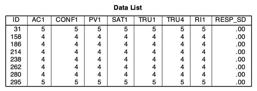
The clearest evidence is item TRU4, "I worry that marketplace X does not keep its promises". This item is reverse-worded: a respondent who trusts Marketplace X should choose a low level. Someone who "Strongly agrees" that they trust Marketplace X (TRU1 = 5) and also "Strongly agrees" that they worry it does not keep its promises (TRU4 = 5) contradicts themselves. This is why a questionnaire should contain at least one reverse-worded item.
To avoid deleting the wrong responses, the syntax first flags each type of problem with a 0/1 variable, counts the flags and only then removes the responses:
COMPUTE ERR_SCREEN = (SL1 = 2).
COMPUTE ERR_ATTENTION = (AC1 <> 2).
COMPUTE ERR_STRAIGHT = (RESP_SD = 0).
COMPUTE EXCLUDE = MAX(ERR_SCREEN, ERR_ATTENTION, ERR_STRAIGHT).
FREQUENCIES ERR_SCREEN ERR_ATTENTION ERR_STRAIGHT EXCLUDE /STATISTICS=NONE.
CROSSTABS /TABLES=ERR_ATTENTION BY ERR_STRAIGHT.

SELECT IF EXCLUDE = 0.
EXECUTE.
The crosstab shows that all 8 straight-lining responses chose 4 or 5 on AC1, so they also failed the attention check. The two detection methods complement each other. Table 1 summarizes the result.
The SELECT IF command permanently deletes the cases that do not meet the condition from the open data set. In the menus, Data > Select Cases offers two choices for unselected cases: filter them temporarily (Filtered) or delete them (Deleted). When in doubt, filter temporarily, and always save the result to a new file.
4. Step 3: Fix data entry errors
A data entry error is a value that cannot occur: outside the scale, outside the valid range set in the codebook or logically inconsistent with another answer. The COUNT command finds every Likert cell outside 1 to 5 in one go:
COUNT OUT_RANGE = CONF1 TO SAT2 SAT3 TO RI4 (LOWEST THRU 0, 6 THRU HIGHEST).
TEMPORARY.
SELECT IF AGE > 60 OR AGE < 18 OR OUT_RANGE > 0.
LIST /VARIABLES=ID AGE OUT_RANGE CONF1 TO SAT2.
TEMPORARY makes the SELECT IF command right after it apply to one procedure only (here LIST), so no data is deleted. The list shows two responses: response 59 with age 230 and response 257 with SAT2 = 55. The valid age range of 18 to 60 comes from the target respondents defined in the codebook.
The best fix is to check the original questionnaire (the paper form or the Google Forms record). If it says 23, change the value to 23; if it says 5, change it to 5. When you cannot check, as with this sample data set, do not guess. Set the cell to missing:
IF (AGE > 60 OR AGE < 18) AGE = $SYSMIS.
RECODE CONF1 TO SAT2 SAT3 TO RI4 (6 THRU HIGHEST = SYSMIS) (LOWEST THRU 0 = SYSMIS).
Also check the logical consistency between items. For example, a respondent who answers "Yes" to the screening question but reports 0 purchases contradicts themselves. In the sample data, all the FREQ = 0 values belong to the 14 "No" responses that were removed, so after Step 2 the minimum of FREQ is 1.
5. Step 4: Assess missing values
Three missing data mechanisms
How you handle missing values depends on why the data are missing. Rubin (1976) distinguished three mechanisms, and Schafer and Graham (2002) explain the consequences of each (Table 2).
Under MCAR, dropping responses with blanks only reduces the sample size and does not bias the results. Under MAR and MNAR, dropping them can leave a sample that is no longer representative.
Measure how much is missing
The NMISS function counts the blank items in each response:
COMPUTE N_BLANK = NMISS(CONF1 TO SAT2, SAT3 TO RI4).
FREQUENCIES N_BLANK /STATISTICS=NONE.
DESCRIPTIVES CONF1 TO SAT2 SAT3 TO RI4 /STATISTICS=MEAN MIN MAX.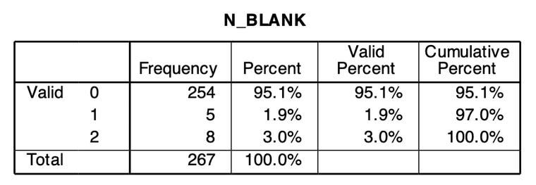
The N column of the DESCRIPTIVES table gives the number of valid values of each item. In total, the sample data have 21 missing cells out of 267 × 20 = 5,340 cells, or 0.39%. The items with the most blanks are CONF3 and RI1, with 3 cells each (1.1%). The 13 responses with at least one blank are 4.9% of the responses, and no response has more than 2 of the 20 items blank.
This is a very low level. Hair et al. (2019) note that missing data under 10% for a single case or variable can generally be ignored if it occurs at random. Tabachnick and Fidell (2019) also observe that when fewer than 5% of the values are missing at random in a large data set, different ways of handling them give nearly the same results.
Check whether the missingness is random
Little (1988) proposed a test of MCAR for multivariate data. SPSS has this test in its Missing Value Analysis module; PSPP does not. A rough check is to compare the responses with blanks and the complete responses on other variables:
COMPUTE HAS_BLANK = (N_BLANK > 0).
T-TEST GROUPS=HAS_BLANK(0 1) /VARIABLES=AGE FREQ.
CROSSTABS /TABLES=GENDER BY HAS_BLANK /STATISTICS=CHISQ.
Results on the sample data:
Gender: the share of responses with blanks does not differ between men, women and other (chi-square(2) = 2.54, p = .280).
Number of purchases: no difference (4.67 versus 4.23 purchases, p = .808).
Age: the group with blanks is younger (26.5 versus 31.7 years). The t-test assuming equal variances is not significant (p = .074), but the Welch test (equal variances not assumed) is (p = .030).
The age result should be reported honestly. The group with blanks has only 13 responses, so the difference may be due to chance. Even if younger respondents do tend to skip items more often (MAR by age), 0.39% of the cells is too small to bias the results noticeably. In your report, give the results of this check instead of simply writing "the data are missing at random".
Choose how to handle missing values
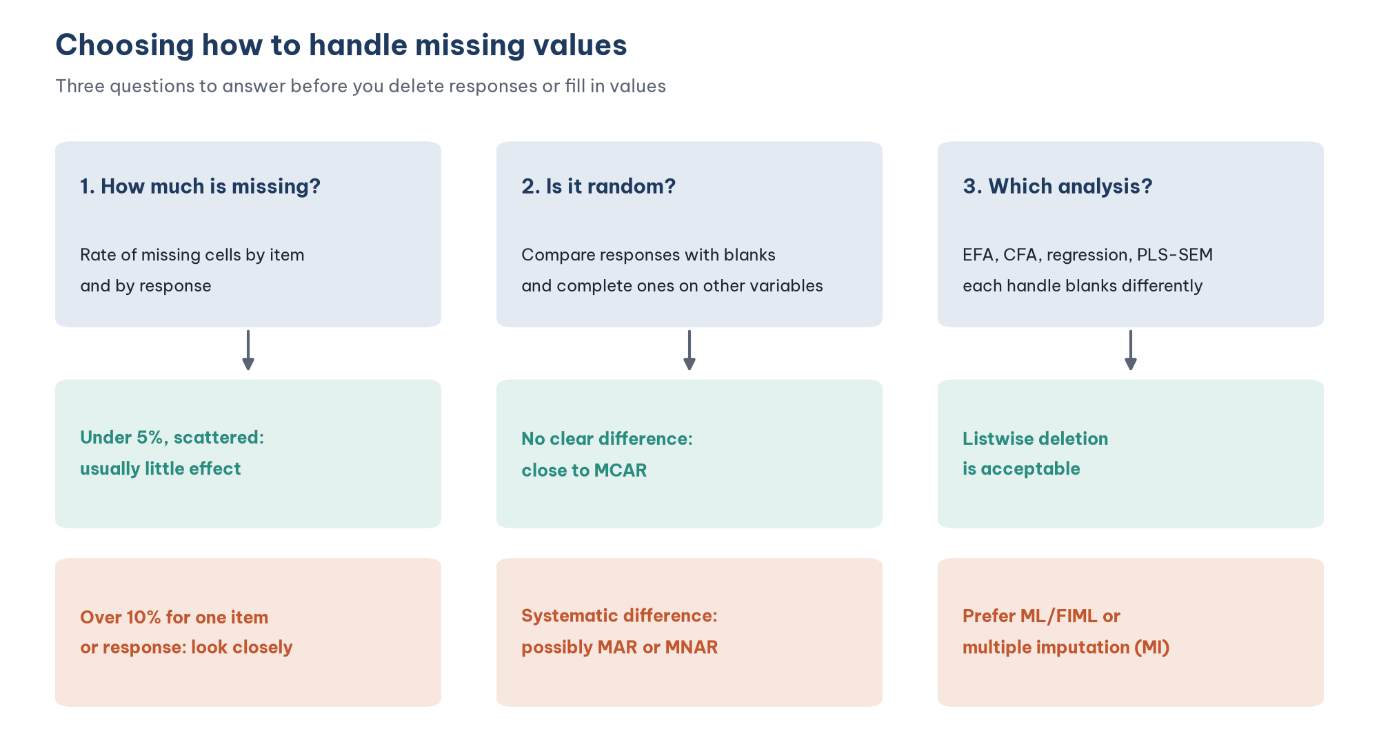
Table 3 compares the common ways of handling missing values.
Newman (2014) recommends ML or MI when the missing rate is substantial, and advises against mean substitution because it artificially shrinks correlations. PSPP does not yet offer ML or MI for missing data. AMOS offers FIML estimation, which is discussed in the CB-SEM posts of this series.
Decision for the sample data: keep all 267 responses, leave the blanks as they are and do not fill in any values. In EFA and regression, the software uses listwise deletion and keeps 254 responses, still above the minimum of 200 for EFA calculated in Post 4. When composite scores are computed in Post 10, "Recoding Variables and Computing Composite Scores in PSPP (SPSS)", the MEAN.3 function averages the items for any response that answered at least 3 of the 4 items of a scale.
6. Step 5: Detect univariate outliers
An outlier is an observation that is clearly different from most of the data. Aguinis et al. (2013) stress the difference between error outliers (to be corrected or removed) and genuine outliers (valid but rare observations that must be considered and reported). Errors were handled in Step 3. This step looks for observations that are valid but unusual.
z-scores
The DESCRIPTIVES command with /SAVE adds a z-score variable (Z + variable name) for each variable. In the menus, check Save Z-scores of selected variables as new variables in the Descriptives dialog (in SPSS, Save standardized values as variables).
DESCRIPTIVES AGE FREQ CONF1 TO SAT2 SAT3 TO RI4 /SAVE /STATISTICS=MEAN STDDEV MIN MAX.
COMPUTE Z_OUTLIER = ANY(1, ABS(ZAGE) > 3.29, ABS(ZFREQ) > 3.29).
Tabachnick and Fidell (2019) suggest a cut-off of |z| > 3.29 (p < .001, two-tailed) for large samples. Result: only response 99 is above the cut-off, with FREQ = 95 and z = 14.44. After the error fix, age has no outliers (its maximum is now 60).
For Likert items, z-scores mean little. The three respondents who chose 1 on CONF2 have |z| of about 3.3, but "Strongly disagree" is a perfectly valid answer on the scale. Do not remove a response just because the respondent chose the lowest or highest level.
Box plots
The EXAMINE command (menu Analyze > Descriptive Statistics > Explore) draws box plots and lists the 5 largest and smallest values:
EXAMINE VARIABLES=FREQ AGE /PLOT=BOXPLOT /STATISTICS=EXTREME(5).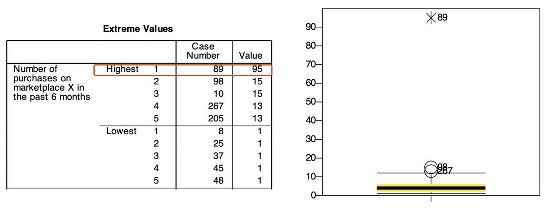
On PSPP and SPSS box plots, a circle marks a value between 1.5 and 3 interquartile ranges (IQR) beyond the edge of the box, and a star marks a value more than 3 IQR beyond it. Note that the Case Number in the table and the labels in the plot are row numbers, not response IDs: after the 33 invalid responses were removed, row numbers no longer match the IDs, and response ID 99 is now in row 89. To label cases by ID, add /ID=ID to the EXAMINE command (GNU Project, n.d.). The labels 98 and 267 overlap in the plot because the two values are close.
Handle univariate outliers
Buying 95 times in 6 months is a lot, but it can happen, for example for a small business owner who buys stock on the marketplace. There is no reason to treat it as an error. Decision for the sample data:
Keep response 99, because its Likert answers are normal and FREQ is not part of the research model.
If you use FREQ in an analysis later, run it twice, with and without response 99, to see whether the results change. Another option is to turn FREQ into groups (1–2, 3–5, 6–10, more than 10 purchases).
Leys et al. (2013) point out that outliers themselves inflate the standard deviation, so the z-score method can miss outliers in small samples. They suggest using the distance from the median measured in median absolute deviations (MAD). With 267 responses and one value as extreme as 95, both methods lead to the same conclusion.
7. Step 6: Detect multivariate outliers
A response may not be unusual on any single item but unusual in its combination of answers. For example, a respondent may strongly disagree that Marketplace X met their expectations (low CONF) but be completely satisfied (high SAT). This type of outlier is detected with the Mahalanobis distance (D²), which measures how far a response is from the centre of the data while taking the correlations between variables into account (Tabachnick & Fidell, 2019).
D² follows a chi-square distribution with degrees of freedom equal to the number of variables. With 20 Likert items, the cut-off at p < .001 is chi-square(20) = 45.31. SPSS computes D² through the linear regression dialog (Save > Mahalanobis). PSPP does not have this option, so the syntax file computes it directly with the MATRIX command, on the 254 complete responses:
MATRIX.
GET X /VARIABLES=CONF1 TO RI4.
GET IDS /VARIABLES=ID.
COMPUTE N = NROW(X).
COMPUTE XC = X - MAKE(N, 1, 1) * CSUM(X) / N.
COMPUTE S = T(XC) * XC / (N - 1).
COMPUTE D2 = RSUM((XC * INV(S)) &* XC).
SAVE {IDS, D2} /OUTFILE=* /VARIABLES=ID MAHAL.
END MATRIX.
COMPUTE P_MAHAL = SIG.CHISQ(MAHAL, 20).
What each line does: XC is the data with each column's mean subtracted, S is the covariance matrix and D2 is the Mahalanobis distance of each response. The SIG.CHISQ function turns D² into a p-value. Before the MATRIX block, the syntax file makes a copy of the data that keeps only the ID and the 20 Likert items of the complete responses. After the block, the distances are merged back into the main data by ID.
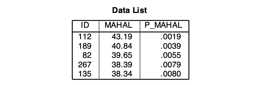
No response is beyond the p < .001 cut-off (the MV_OUTLIER flag is 0 for all 254 complete responses). The result was checked again in Python (numpy), which gives the same D² values. Response 112 has the largest D² because its answers are inconsistent within the same scale: CONF1 = 1 but CONF3 = 4; PV1 = 5 but PV4 = 3. These are still valid answers, so there is no reason to remove it.
When a response is beyond the cut-off, do not delete it automatically. Open it, find out why it is different and run the main analysis with and without it. If the conclusions do not change, keep it and report it. If they change, report both results and the reason for your choice (Aguinis et al., 2013). Also note that if you recompute D² after deleting outliers, other responses often become "new outliers", because the centre and the covariances change. So check once only; do not repeat the check until the data look "clean".
8. Step 7: Save the clean data and keep a log
The last step saves the data set as a new file and drops the intermediate variables:
SAVE OUTFILE='../data/marketplace_x_clean.sav'
  /DROP=OUT_RANGE ERR_SCREEN ERR_ATTENTION ERR_STRAIGHT EXCLUDE HAS_BLANK Z_OUTLIER
        ZAGE ZFREQ ZCONF1 TO ZRI4.
The file marketplace_x_clean.sav has 267 responses and keeps three variables that are useful in later posts: RESP_SD (standard deviation within the response), N_BLANK (number of blank items) and MAHAL (Mahalanobis distance, with its p-value P_MAHAL and the flag MV_OUTLIER; these are empty for the 13 responses with blanks). This is the data set used throughout the following SPSS posts.
Alongside the data file, keep a data cleaning log. The methods section of a thesis or article needs these numbers (Table 4).
A sample sentence for the methods section: "Of the 300 responses collected, 33 (11%) were removed because they failed the screening question (14 responses) or the attention check (19 responses, 8 of which gave the same answer to every item). Two out-of-range values were set to missing. Missing data accounted for 0.39% of the scale cells; no response had more than 2 of the 20 items missing. No multivariate outliers were found with the Mahalanobis distance (p < .001). The analysis sample consisted of 267 responses."
Five common mistakes
Looking for outliers before removing invalid responses, so the means and standard deviations used for the z-scores are distorted.
Treating every outlier as an error and deleting it. Only impossible values are errors. Genuine outliers must be considered and reported.
Filling in missing values with the mean for convenience, which shrinks the variances and the correlations between variables.
Overwriting the original data file, so the cleaning decisions can no longer be checked or changed.
Not reporting the cleaning process, so readers do not know how 300 questionnaires became a sample of 267.
Frequently asked questions
Should I remove responses that were completed too quickly?
Yes, if you have timing data. Google Forms records only the time a response was submitted, not the time it was started, so you cannot compute the completion time. Other survey platforms usually record the duration. Huang et al. (2012) suggest a cut-off of 2 seconds per item: a respondent faster than this is unlikely to have read the items. If you apply it, state the cut-off in your report.
Is removing 11% of the responses too much?
It is not unusual for online surveys. What matters is that the removal criteria are decided in advance and applied consistently, not chosen after you have seen the results of the analysis. This is also why Post 4 recommends distributing more questionnaires than the target sample size, allowing for about 15% to be discarded.
Do SmartPLS and AMOS handle missing values themselves?
Yes, each in its own way. SmartPLS offers mean replacement, casewise (listwise) deletion or pairwise deletion. AMOS uses FIML when you choose to estimate means and intercepts. Cleaning the data first in PSPP or SPSS means you know your data well before you hand it to these programs.
References
Aguinis, H., Gottfredson, R. K., & Joo, H. (2013). Best-practice recommendations for defining, identifying, and handling outliers. Organizational Research Methods, 16(2), 270–301. https://doi.org/10.1177/1094428112470848
Curran, P. G. (2016). Methods for the detection of carelessly invalid responses in survey data. Journal of Experimental Social Psychology, 66, 4–19. https://doi.org/10.1016/j.jesp.2015.07.006
Enders, C. K. (2010). Applied missing data analysis. Guilford Press.
Free Software Foundation. (2026). GNU PSPP (Version 2.1.2) [Computer software]. https://www.gnu.org/software/pspp/
GNU Project. (n.d.). GNU PSPP manual. Retrieved November 19, 2026, from https://www.gnu.org/software/pspp/manual/
Hair, J. F., Black, W. C., Babin, B. J., & Anderson, R. E. (2019). Multivariate data analysis (8th ed.). Cengage Learning.
Huang, J. L., Curran, P. G., Keeney, J., Poposki, E. M., & DeShon, R. P. (2012). Detecting and deterring insufficient effort responding to surveys. Journal of Business and Psychology, 27(1), 99–114. https://doi.org/10.1007/s10869-011-9231-8
Leys, C., Ley, C., Klein, O., Bernard, P., & Licata, L. (2013). Detecting outliers: Do not use standard deviation around the mean, use absolute deviation around the median. Journal of Experimental Social Psychology, 49(4), 764–766. https://doi.org/10.1016/j.jesp.2013.03.013
Little, R. J. A. (1988). A test of missing completely at random for multivariate data with missing values. Journal of the American Statistical Association, 83(404), 1198–1202. https://doi.org/10.1080/01621459.1988.10478722
Meade, A. W., & Craig, S. B. (2012). Identifying careless responses in survey data. Psychological Methods, 17(3), 437–455. https://doi.org/10.1037/a0028085
Newman, D. A. (2014). Missing data: Five practical guidelines. Organizational Research Methods, 17(4), 372–411. https://doi.org/10.1177/1094428114548590
Rubin, D. B. (1976). Inference and missing data. Biometrika, 63(3), 581–592. https://doi.org/10.1093/biomet/63.3.581
Schafer, J. L., & Graham, J. W. (2002). Missing data: Our view of the state of the art. Psychological Methods, 7(2), 147–177. https://doi.org/10.1037/1082-989X.7.2.147
Tabachnick, B. G., & Fidell, L. S. (2019). Using multivariate statistics (7th ed.). Pearson.
Discussion about this post