Sample Size Calculation for EFA, Regression, PLS-SEM and CB-SEM
How to justify the sample size for EFA, regression, PLS-SEM, CB-SEM and mediation with G\*Power, Green’s rule and the inverse square root method


Key takeaways
The sample size follows from the analysis techniques, the complexity of the model and the expected effect size; compute it for each technique and take the largest value.
The Cochran and Yamane formulas estimate a population proportion; they are not a basis for testing a model.
For the example regression with 3 predictors, the minimum ranges from 36 to 550 depending on the effect size, so take the effect size from earlier studies.
For PLS-SEM, drop the 10-times rule and use the inverse square root method: a smallest path coefficient of 0.20 needs 155 observations.
The example model needs at least 200 observations (EFA, 10:1); a target of 250 valid responses with 15% invalid questionnaires means distributing 300.
"How large should my sample be?" is probably the most frequent question when you write a research proposal. The usual answers, such as "200 is enough" or "five times the number of items", may be right for one study and wrong for another. There is no single number, because the sample size depends on the analysis techniques you will use, the complexity of the model and the size of the effect you want to detect.
This post presents the methods for determining the sample size for each technique commonly used in a thesis, then applies all of them to the example model of this series: customers' repurchase intention on an online marketplace, Marketplace X, with 5 constructs and 6 hypotheses (see Post 2, "The 7-Step Quantitative Research Process"). Every number in this post is computed with an accompanying Python script, so you can check it and recompute it for your own study.
Sample script. The Python script that computes every number in this post,
sample_size.py, and its output are in the research-data-analysis repository on GitHub (folderscripts/). Download the whole repository with Code > Download ZIP.
1. Why sample size matters
A sample that is too small causes three problems:
Missing real effects. A small sample lowers statistical power, the probability of detecting an effect when that effect really exists. A hypothesis may be rejected only because the sample was not large enough, not because the relationship does not exist.
Unstable estimates. Regression coefficients, factor loadings and path coefficients vary a lot between small samples.
Models that do not converge. In CB-SEM, a small sample can easily make the algorithm fail to converge or produce impossible estimates, such as negative variances (Kline, 2023).
A sample that is too large also has a downside: it costs more, and almost every effect, however small, becomes statistically significant. With a large sample, it is therefore even more important to report effect sizes.
2. Four factors that determine the sample size
In principle, the sample size follows from four factors (Cohen, 1992):
Significance level (alpha): the probability of concluding that there is an effect when there is none. The usual choice is alpha = 0.05.
Power (1 − beta): the probability of detecting an effect when the effect is real. The usual level is 0.80.
Expected effect size: the smaller the effect, the larger the sample needed to detect it. Cohen (1992) proposed conventional small, medium and large values for each type of test; for multiple regression, the three values are f² = 0.02, 0.15 and 0.35.
Model complexity: the number of predictors, constructs and parameters to estimate.
"Rules of thumb" such as 5:1 or 10:1 are in fact rough substitutes for a calculation based on these four factors. They are useful for a quick check, but they should not be your only justification.
3. The procedure for determining the sample size
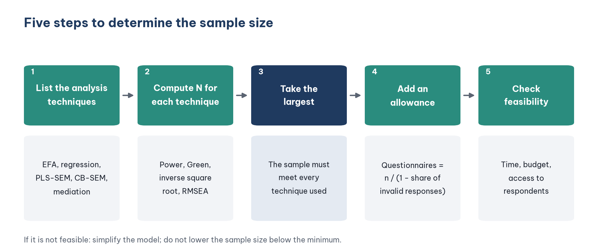
List the analysis techniques you will use, as decided when you built the model (for example EFA, regression, PLS-SEM).
Compute the minimum sample size for each technique with the appropriate method from Section 4.
Take the largest value among the requirements, because the sample must meet every technique.
Add an allowance for invalid questionnaires. If you expect to discard 15% of the questionnaires, the number to distribute is n / (1 − 0.15).
Check feasibility: time, budget and access to respondents. If the target is not feasible, consider simplifying the model rather than lowering the sample size below the minimum.
4. Methods for each technique
4.1. Estimating a proportion or a mean: the Cochran and Yamane formulas
These two formulas are widely used in student theses, but they are often used for the wrong purpose. They are designed to estimate a population proportion with a given margin of error, for example the share of satisfied customers (Cochran, 1977; Yamane, 1967):
Cochran (large population): n = z² × p(1 − p) / e². With 95% confidence (z = 1.96), p = 0.5 and a margin of error e = 5%, n = 385 (384.16 rounded up).
Yamane (known population size N): n = N / (1 + N × e²). With e = 5%, N = 2,000 gives n = 334; N = 100,000 gives n = 399.
These formulas do not take into account the number of variables, the number of hypotheses or the effect size, so they are not a suitable basis for testing a model. If your study has both a descriptive objective (estimating a proportion) and a model-testing objective, compute both and take the larger value. Note also that the Yamane formula assumes simple random sampling; applying it to a convenience sample does not make the sample representative.
4.2. Exploratory factor analysis (EFA)
Hair et al. (2019) recommend a minimum sample size of 50, preferably 100 or more, with a ratio of at least 5 observations per item, and preferably 10 observations per item.
Applied to the example model: 5 constructs × 4 items = 20 items. The 5:1 ratio gives 100 observations; the 10:1 ratio gives 200 observations.
4.3. Multiple regression: Green's rule and power analysis
Green's rule (1991) gives two numbers, depending on what you test:
Testing the whole model (R²): N of at least 50 + 8*m*, where m is the number of predictors.
Testing each individual predictor: N of at least 104 + m.
Take the larger number, because a thesis usually tests both.
Power analysis with G*Power gives a more precise result, because it computes the sample size directly from the four factors in Section 2 (Faul et al., 2009). The settings in G*Power are:
Applied to the example model: the SPSS posts of this series regress repurchase intention on 3 predictors (perceived value, satisfaction and trust), so m = 3.
The table shows how strongly the effect size matters: for the same model, the minimum sample size ranges from 36 to 550. Choose the effect size based on the results of earlier studies; do not choose the "large" value only to get a small sample.
4.4. PLS-SEM: drop the 10-times rule and use the inverse square root method
The 10-times rule (a sample size of 10 times the largest number of arrows pointing at a construct) used to be very popular. However, PLS-SEM authors advise against it, because it ignores the effect size and often gives a sample that is too small (Hair et al., 2022). In the example model, the repurchase intention construct receives 3 arrows, so the 10-times rule gives only 30 observations, a number that is clearly not enough.
The inverse square root method of Kock and Hadaya (2018) is the recommended alternative. At a 5% significance level and 80% power:
nₘᵢₙ > (2.486 / |pₘᵢₙ|)²
where pₘᵢₙ is the smallest path coefficient that you expect to be statistically significant. Take this value from earlier studies that used a similar model.
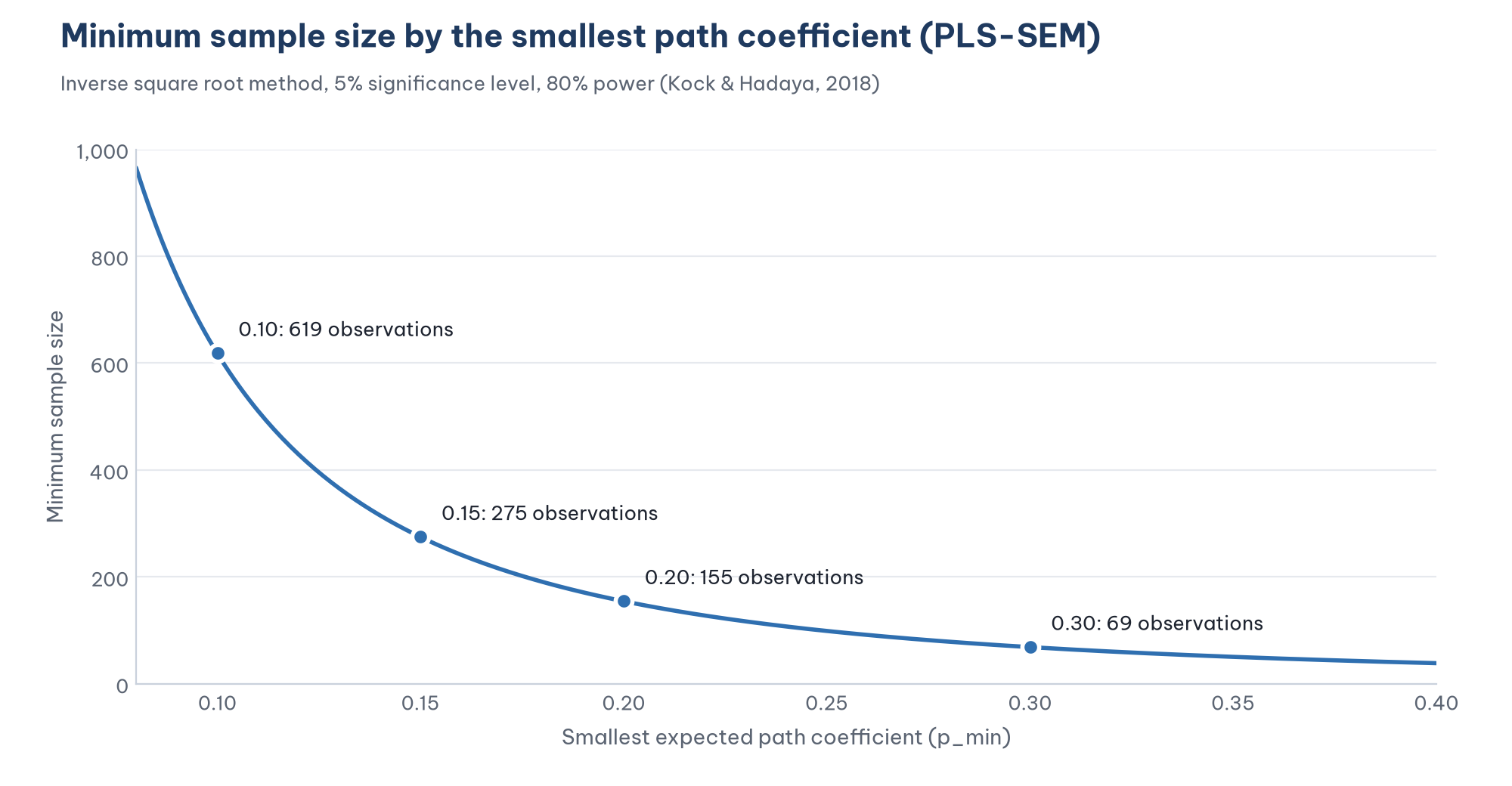
Applied to the example model: suppose that in earlier studies, the smallest path coefficient of similar relationships is about 0.20 (an assumed value for illustration). The minimum sample size is 155 observations.
4.5. CB-SEM: from rules of thumb to power analysis
For CB-SEM, there are three approaches, from simple to rigorous:
Ratio of observations to parameters (N:q). Kline (2023) mentions an ideal ratio of 20 observations per free parameter, or 10:1 as a less desirable level, but also notes that this is only a rough rule of thumb. A CFA model with 5 constructs and 20 items has 50 free parameters (15 loadings, 20 error variances, 5 factor variances and 10 covariances between factors). The 10:1 ratio gives 500 observations and the 20:1 ratio gives 1,000 observations, far more than most theses can collect.
Guidelines based on model characteristics. Hair et al. (2019) suggest that a model with 5 or fewer constructs, each measured by more than 3 items with high communalities, can be estimated with a sample of about 100 to 150, whereas a model with many constructs (more than 6) and low communalities may need more than 500.
Power analysis based on RMSEA. MacCallum et al. (1996) proposed computing the sample size for testing whether a model has close fit: the hypothesis RMSEA = 0.05 is compared with RMSEA = 0.08. The sample size depends on the degrees of freedom (df) of the model. For the example CFA model (df = 160), the minimum sample size for a power of 0.80 is 97 observations. The more degrees of freedom a model has, the smaller the sample needed for this test, so this number must be considered alongside the other requirements.
The simulations of Wolf et al. (2013) show that the sample size needed for SEM varies widely, from about 30 to 460, depending on the model structure, the number of items, the size of the loadings and the presence of a mediator. This is why you should not apply one fixed number to every model.
4.6. Mediation analysis
The example model has satisfaction as a mediator. The indirect effect equals the product of two path coefficients (a × b), so it is usually smaller than each component effect and needs a larger sample to detect. The simulations of Fritz and MacKinnon (2007) with the percentile bootstrap, the default type of bootstrap in many programs, show that a power of 0.80 requires:
About 78 observations when both paths a and b are medium.
About 558 observations when both paths are small.
So if earlier studies show that the effect through satisfaction is small, a sample of a few hundred observations may still not be enough to detect the indirect effect.
5. Summary for the example model
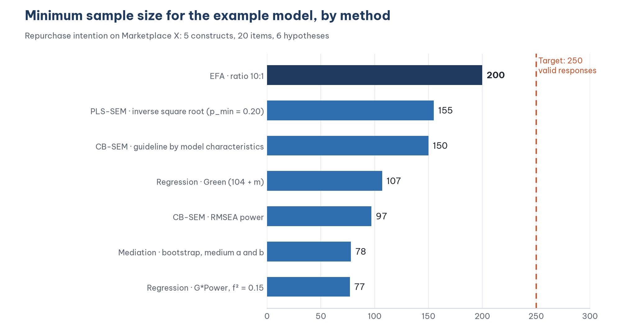
Applying the procedure of Section 3:
The largest requirement is 200 (EFA with the 10:1 ratio).
Choose a target of 250 valid responses for an extra safety margin. With 250 observations, PLS-SEM can detect a smallest path coefficient of about 0.16, which is smaller than the assumed 0.20.
Expect to discard 15% of the questionnaires because they fail the screening question or are answered carelessly: the number to distribute is 250 / 0.85 = 294.1, rounded up to 295 and then to 300 questionnaires.
6. Writing the sample size section of your methods chapter
Examiners rarely ask only "how large is the sample"; they ask "what is it based on". A good paragraph states the technique, the calculation method, the input values and the result. For example:
The study uses EFA and PLS-SEM. With 20 items, EFA requires at least 200 observations under the 10:1 ratio (Hair et al., 2019). For PLS-SEM, the inverse square root method (Kock & Hadaya, 2018) with an expected smallest path coefficient of 0.20, based on earlier studies, gives a minimum sample size of 155. The study set a target of 250 valid responses. Allowing for 15% invalid questionnaires, 300 questionnaires were distributed.
Five common mistakes
Using the Yamane or Cochran formula as the only justification for a model-testing study. These formulas serve to estimate a proportion; they ignore the number of variables and the effect size.
Applying the 10-times rule to PLS-SEM. This rule often gives a sample that is too small and is no longer recommended.
Choosing a "large" effect size to get a small sample, while earlier studies show that the effect is only medium or small.
Computing the sample size for the questionnaires distributed instead of the valid responses. The minimum sample size is the number of observations left after data cleaning.
Believing that a large sample makes up for a non-representative one. A convenience sample of 1,000 people is still a convenience sample. Sample size solves the problem of power, not the problem of representativeness.
Frequently asked questions
What if I collect fewer responses than my target?
If the number of valid responses still meets the minimum of every technique you use, report the actual number and discuss its effect on power in the limitations section. If it falls below the minimum, collect more data before you analyze, instead of switching to a rule that gives a smaller number.
Is a larger sample always better?
Not necessarily. A sample larger than needed costs more and makes even very small effects statistically significant. Rely on the calculated sample size, and always report effect sizes.
Where do I get the effect size or the smallest path coefficient?
From earlier studies that used a similar model and context, which is the literature review matrix you built during the literature review. If there are none, use the conventional medium value of Cohen (1992) and state this assumption clearly.
References
Cochran, W. G. (1977). Sampling techniques (3rd ed.). Wiley.
Cohen, J. (1992). A power primer. Psychological Bulletin, 112(1), 155–159. https://doi.org/10.1037/0033-2909.112.1.155
Faul, F., Erdfelder, E., Buchner, A., & Lang, A.-G. (2009). Statistical power analyses using G*Power 3.1: Tests for correlation and regression analyses. Behavior Research Methods, 41(4), 1149–1160. https://doi.org/10.3758/BRM.41.4.1149
Fritz, M. S., & MacKinnon, D. P. (2007). Required sample size to detect the mediated effect. Psychological Science, 18(3), 233–239. https://doi.org/10.1111/j.1467-9280.2007.01882.x
Green, S. B. (1991). How many subjects does it take to do a regression analysis? Multivariate Behavioral Research, 26(3), 499–510. https://doi.org/10.1207/s15327906mbr2603_7
Hair, J. F., Black, W. C., Babin, B. J., & Anderson, R. E. (2019). Multivariate data analysis (8th ed.). Cengage Learning.
Hair, J. F., Hult, G. T. M., Ringle, C. M., & Sarstedt, M. (2022). A primer on partial least squares structural equation modeling (PLS-SEM) (3rd ed.). SAGE Publications.
Kline, R. B. (2023). Principles and practice of structural equation modeling (5th ed.). Guilford Press.
Kock, N., & Hadaya, P. (2018). Minimum sample size estimation in PLS-SEM: The inverse square root and gamma-exponential methods. Information Systems Journal, 28(1), 227–261. https://doi.org/10.1111/isj.12131
MacCallum, R. C., Browne, M. W., & Sugawara, H. M. (1996). Power analysis and determination of sample size for covariance structure modeling. Psychological Methods, 1(2), 130–149. https://doi.org/10.1037/1082-989X.1.2.130
Wolf, E. J., Harrington, K. M., Clark, S. L., & Miller, M. W. (2013). Sample size requirements for structural equation models: An evaluation of power, bias, and solution propriety. Educational and Psychological Measurement, 73(6), 913–934. https://doi.org/10.1177/0013164413495237
Yamane, T. (1967). Statistics: An introductory analysis (2nd ed.). Harper & Row.
Discussion about this post