Confirmatory Factor Analysis (CFA) in JASP: Output and Mardia's Test
Run a five-factor CFA in free JASP with FIML, read the loadings, correlations and modification indices, then test multivariate normality with Mardia’s coefficient


Key takeaways
A CFA states in advance which items measure which factor; five factors with 20 items give 160 degrees of freedom.
In JASP, FIML keeps all 267 respondents, and the modification indices come from the same run.
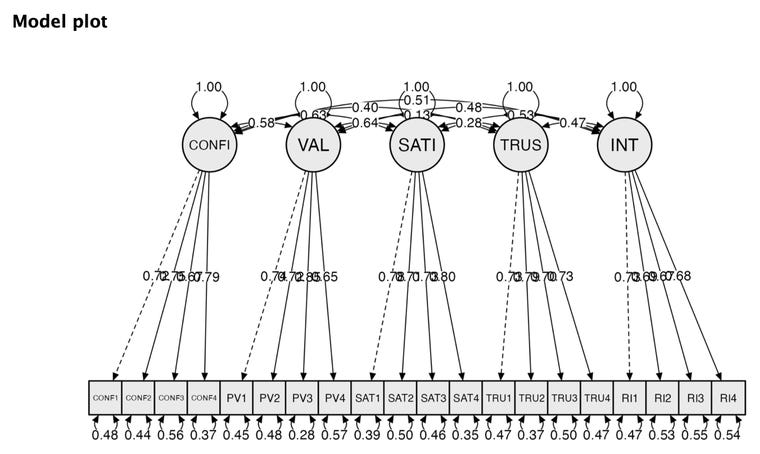
All standardized loadings are significant and range from 0.65 to 0.85; the highest factor correlation is 0.64.
Small modification indices without a theoretical reason are no basis for changing the model.
Mardia's test is in the SEM module, not the Factor module; a critical ratio of 4.62 is below Bentler's cutoff of 5.
Post 12, "Exploratory Factor Analysis (EFA) in PSPP (SPSS)" used EFA to explore how the 20 items group together and found the five factors of the design. Confirmatory factor analysis (CFA) works the other way round: you state in advance which items measure which concept, then test whether the data support that structure (Brown, 2015). CFA is a required step before SEM: if the measurement model does not hold up, conclusions about the hypotheses in the structural model cannot be trusted (Anderson & Gerbing, 1988).
This post runs a CFA for the five scales of the Marketplace X model (20 items), reads the core results and carries out Mardia's test of multivariate normality, as promised in the FAQ of Post 9, "Descriptive Statistics in PSPP (SPSS)". The next three posts go deeper into each group of indices: model fit (Post 23, "SEM Model Fit Indices in JASP"), CR and AVE (Post 24, "Composite Reliability (CR) and Average Variance Extracted (AVE) in JASP") and discriminant validity (Post 25, "Convergent and Discriminant Validity in JASP").
Sample data and scripts. The data files and scripts for this post are in the research-data-analysis repository on GitHub (folder
data/andscripts/). Download the whole repository with Code > Download ZIP.
About the figures and numbers. Figures 1, 2 and 10 to 12 are real screenshots of JASP 0.99.0 (JASP Team, 2026) on macOS, taken in November 2026 with the file
marketplace_x_sem.savprepared in Post 21, "Preparing and Connecting Data from SPSS to JASP" (in thedata/folder of the repository). Figures 5 to 8 and 13 are real JASP output, exported with Export Results and cropped; nothing in them is changed. The numbers were checked with the R package lavaan (Rosseel, 2012) in the scriptcfa_5_factors.R(folderscripts/of the repository), which also computes the results JASP does not provide (item skewness and kurtosis, Mahalanobis distances, standardized residuals and the Bollen-Stine bootstrap). In AMOS, the same CFA is drawn with Plugins > Draw Covariances for the 10 factor covariances and run with Analyze > Calculate Estimates. Modification indices, Tests for normality and outliers and the Bollen-Stine bootstrap do not run when the data have missing cells (Byrne, 2016), so AMOS users run these checks on the 254 complete respondents (marketplace_x_sem_complete.sav) and take the reported estimates from a run with Estimate means and intercepts on all 267.
1. The measurement model to be tested
In a CFA, each item loads on only one factor, the measurement errors are uncorrelated and every pair of factors is allowed to correlate (10 covariances). The factor names differ from every column name in the data file (Posts 20 and 21).
With 20 items, the data contain 20 × 21 / 2 = 210 variances and covariances. The model estimates 50 parameters: 15 loadings (the other 5 are fixed to 1), 20 error variances, 5 factor variances and 10 covariances between the factors. The degrees of freedom are 210 − 50 = 160.
2. Running the CFA in JASP
Specify the five factors
Open the file
marketplace_x_sem.sav(the items are already Scale variables after the preparation in Post 21) and choose Factor > Confirmatory Factor Analysis.Move CONF1 to CONF4 into the Factor 1 box, double-click the box title and rename it CONFIRM.
Click the green plus button below the factor boxes to add a new factor; repeat for VALUE, SATISF, TRUST and INTENT (Figure 1).
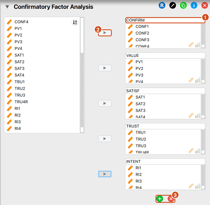
By default, JASP lets every pair of factors correlate and fixes the first loading of each factor to 1 (section Model Options), as AMOS does. In the variable list on the left, items already assigned to a factor stay visible, because JASP allows an item to load on several factors; take care not to put one item into two factors by mistake.
Choose the options
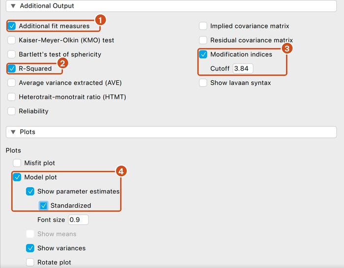
Unlike AMOS, JASP computes modification indices with FIML, so a single run with all 267 respondents is enough. The Information criteria table confirms that FIML is in use: it reports 70 free parameters, the 50 parameters above plus 20 item intercepts.
3. Reading the output in six steps
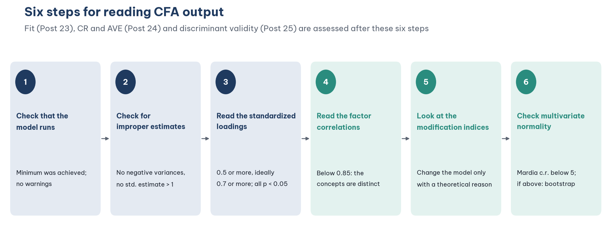
Step 1. Check that the model runs
The Chi-square test table in the results pane on the right shows the chi-square with the note The estimator is ML. If lavaan fails to converge or produces improper estimates, JASP shows a red warning just below the title of the analysis.
With the sample data the model runs normally. Chi-square = 134.293; df = 160; p = 0.931; CFI = 1.000; RMSEA = 0.000; SRMR = 0.032. Post 23 analyzes these indices; here it is enough to note that the model fits the data. The near-perfect fit arises because the data were simulated from exactly this structure (Post 19, "What Is AMOS? CB-SEM and When to Use It Instead of SPSS").
Step 2. Check for improper estimates
Look for two warning signs (Kline, 2023):
Negative variances of an error or a factor (a Heywood case).
Standardized estimates greater than 1 in absolute value.
Neither occurs in the sample data: the smallest standardized error variance is 0.28 (PV3, Residual variances table).
Step 3. Read the standardized loadings
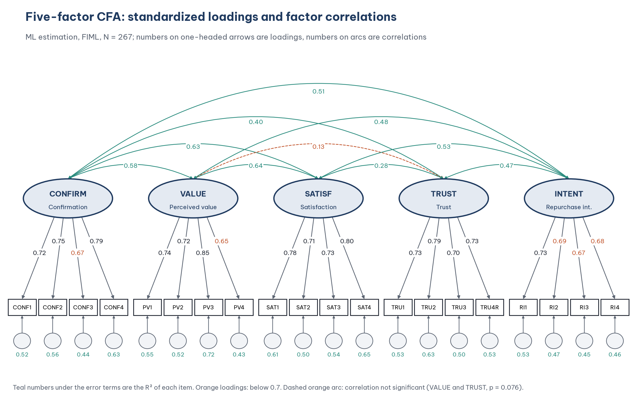
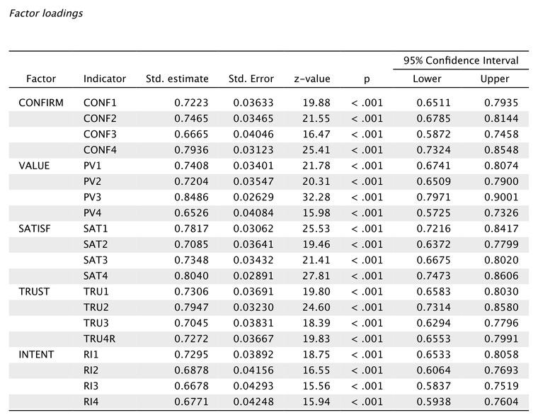
Every loading is significant (p < 0.001; the z-values in the standardized table range from 15.56 to 32.28).
Every standardized loading is 0.65 or higher. The usual minimum is 0.5, and 0.7 or higher is ideal (Hair et al., 2019). Five items lie between 0.65 and 0.69 (CONF3, PV4, RI2, RI3, RI4). This is acceptable; do not drop an item only because its loading is below 0.7 if the scale still meets the CR and AVE criteria (Post 24) and the item matters for content.
R² is the square of the standardized loading: 72% of the variance of PV3 is explained by Perceived value, but only 43% of PV4.
The order of the loadings is quite similar to the EFA in Post 12 (for example, PV3 is the highest in the Perceived value scale), but the values are not identical: unlike EFA, CFA does not allow items to have secondary loadings on other factors.
Step 4. Read the correlations between the factors
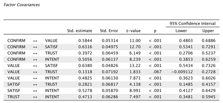
The highest correlation is 0.64 (Perceived value and Satisfaction), well below the cutoff of 0.85 often used to warn that two concepts overlap (Kline, 2023). Post 25 tests discriminant validity in more detail with the Fornell-Larcker criterion and HTMT.
Perceived value and Trust are almost uncorrelated (0.13; p = 0.067 in JASP's standardized table, 95% CI [−0.009, 0.273]), in line with the Pearson correlation between the mean scores in Post 13, "Pearson Correlation in PSPP (SPSS)" (r = 0.12; p = 0.051). The test of the unstandardized covariance in the R script gives p = 0.076, the value AMOS reports; both are above 0.05.
The correlations in the CFA are higher than the correlations between the mean scores in Post 13, because CFA removes measurement error (Post 19).
Step 5. Look at the modification indices
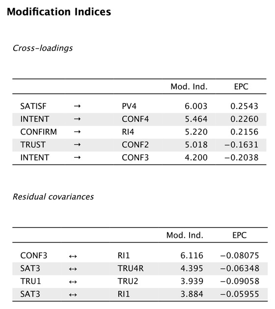
A modification index (MI) estimates how much the chi-square would drop if a fixed parameter were freed (Brown, 2015). JASP lists nine MIs above the cutoff of 3.84; the five largest are:
JASP prints the expected change in unstandardized form. In the Cross-loadings table, a row such as "SATISF, PV4" means the factor SATISF would get an extra loading on item PV4.
Do not modify the model on the basis of these MIs. Three reasons:
The MIs are small. The largest, 6.12, is only just above 3.84 (the critical chi-square with 1 degree of freedom at the 0.05 level). With 190 parameters that could be freed, a few MIs above 3.84 by chance are normal.
There is no theoretical reason. Nothing suggests that the error of an item about delivery service (CONF3) should correlate with the error of an item about the plan to keep buying (RI1).
The model already fits well. Further changes would only fit the model to the peculiarities of this sample and would be hard to replicate in another one (MacCallum et al., 1992).
An additional check is the standardized residuals (computed by the R script): only 1 of the 190 residuals exceeds 2.58 in absolute value (the largest is 2.82), so no pair of items is poorly reproduced by the model.
4. Testing multivariate normality
ML estimation assumes the data are multivariate normal. When multivariate kurtosis is high, the chi-square is inflated and the standard errors are underestimated, which leads to rejecting the model and finding significance more often than is warranted (Kline, 2023). This is why the FAQ of Post 9 recommended checking normality at the CFA stage rather than testing each item with Shapiro-Wilk.
Distribution of each item
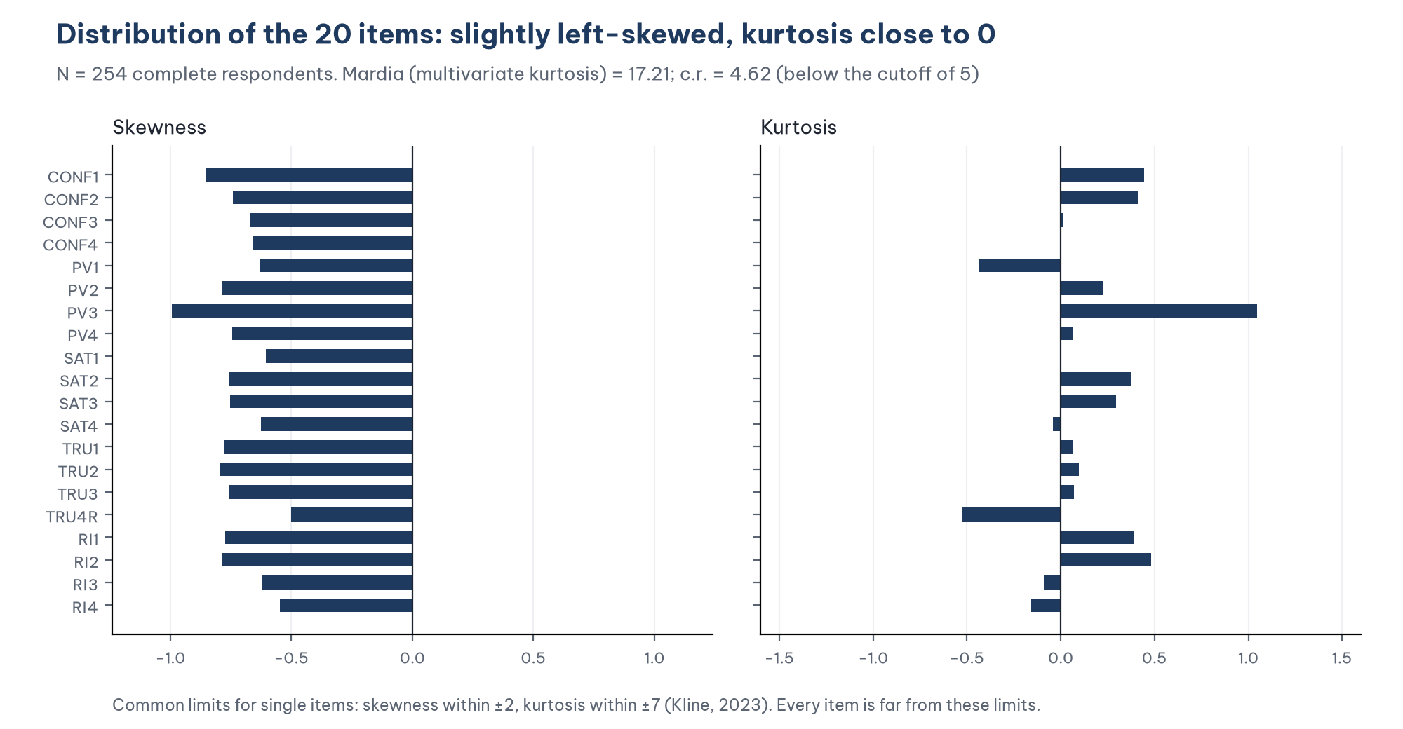
Skewness ranges from −0.99 (PV3) to −0.50 (TRU4R): every item is slightly left-skewed, because most respondents chose "Agree". Kurtosis ranges from −0.53 to 1.05.
Both are far from the usual limits for single variables: |skewness| < 2 and |kurtosis| < 7 (Kline, 2023).
The critical ratios (c.r.) of skewness range from −6.46 to −3.27, all beyond 1.96. This does not mean the distributions are severely skewed: the c.r. is the skewness divided by its standard error, and the standard error shrinks as the sample grows, so with 254 respondents even a small skewness gives a large c.r. Read the size of the skewness, not the c.r. of each item.
Mardia's coefficient
The Factor module of JASP has no Mardia's test. The SEM module does:
Enable the SEM module with the plus button at the right end of the toolbar and tick SEM.
Choose SEM > Structural Equation Modeling (Figure 10).
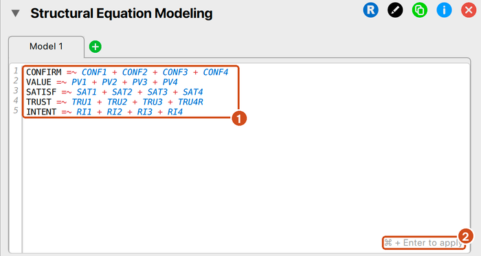
Type the model in lavaan syntax into the editor and press Cmd+Enter (Ctrl+Enter on Windows) (Figure 11):
CONFIRM =~ CONF1 + CONF2 + CONF3 + CONF4
VALUE =~ PV1 + PV2 + PV3 + PV4
SATISF =~ SAT1 + SAT2 + SAT3 + SAT4
TRUST =~ TRU1 + TRU2 + TRU3 + TRU4R
INTENT =~ RI1 + RI2 + RI3 + RI4
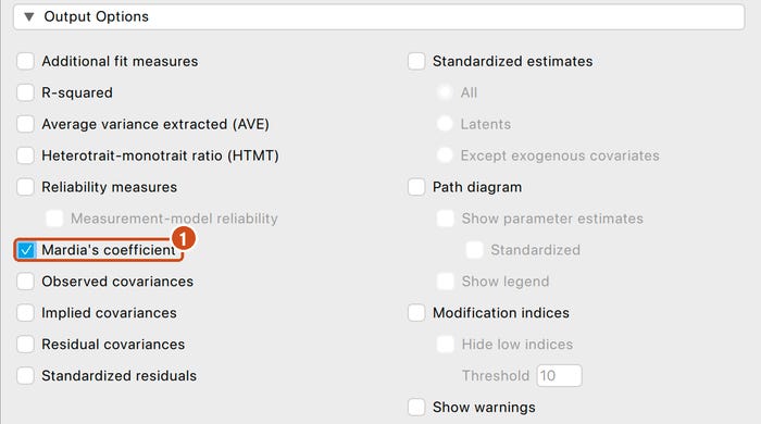
Tick Mardia's coefficient in the Output Options section (Figure 12).

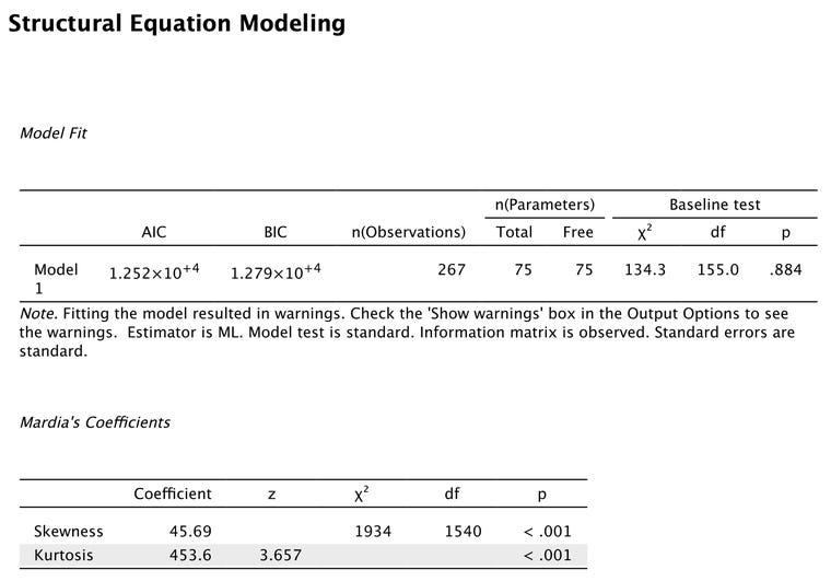
JASP computes Mardia's coefficients on the 254 complete respondents (the R script reproduces both values from these 254 rows): the kurtosis coefficient (Kurtosis) = 453.6, z = 3.657. The value 453.6 is Mardia's b2; its expected value for normal data is p(p + 2) = 20 × 22 = 440. AMOS reports the excess over 440, so to compare with the way theses using AMOS usually report it, take 453.6 − 440 = 13.6. With the original formula of Mardia (1970), which uses the covariance matrix divided by N instead of N − 1 as JASP does:
Multivariate kurtosis = 17.21; critical ratio = 4.62.
Bentler (2005) suggests treating the data as not multivariate normal when the critical ratio of Mardia's coefficient is greater than 5. At 4.62, the sample data are below that cutoff, so ML estimation is appropriate.
JASP's z = 3.657 is lower than 4.62 because of the different denominator described above; both are below 5. The JASP table also has a test of multivariate skewness (Skewness: chi-square = 1934; df = 1540; p < 0.001). This test is very sensitive to sample size and to the common direction of skew in Likert scales. ML estimation is more sensitive to kurtosis than to skewness, which is why Bentler's rule is based on kurtosis (Kline, 2023). Still, significant skewness is a reason to double-check with the Bollen-Stine bootstrap below.
A further note: the Model Fit table of the SEM module shows df = 155 instead of 160 (chi-square = 134.3; p = 0.884). With FIML, the SEM module of JASP 0.99.0 also estimates the means of the five factors (the Intercepts table shows them as approximately 0); the chi-square does not change. The table also carries a note that fitting the model resulted in warnings. For these reasons, this post uses the Factor module for the main CFA results and the SEM module only for Mardia's coefficients.
Multivariate outliers
The Mahalanobis distance (d*²) measures how far each respondent is from the centroid on all 20 items at once. The five respondents farthest from the centroid have *d*² from 38.65 to 43.53 (IDs 112, 189, 82, 267 and 135), with *p from 0.002 to 0.007. Nobody has p < 0.001, the usual cutoff for a multivariate outlier (Tabachnick & Fidell, 2019), which agrees with the conclusion of Post 8, "Data Cleaning in PSPP (SPSS)".
The Bollen-Stine bootstrap
When the critical ratio of Mardia's coefficient exceeds 5, you can keep the ML estimates but replace the p-value of the chi-square with the Bollen-Stine bootstrap p-value (Bollen & Stine, 1992). This method transforms the data so that the model fits them exactly, draws 2000 bootstrap samples and counts the proportion of samples with a chi-square larger than the observed value.
The sample data do not need it, but the post runs it as an illustration: on the 254 complete respondents, chi-square = 137.05 and the Bollen-Stine p = 0.922 (2000 samples), close to the p = 0.931 of the usual test. The conclusion about fit does not change.
JASP 0.99.0 has no Bollen-Stine option in its interface; the script cfa_5_factors.R in the repository computes it directly with lavaan. AMOS users choose it under Analysis Properties > Bootstrap.
5. Reporting the CFA in a thesis
A confirmatory factor analysis with maximum likelihood estimation and FIML for missing data (N = 267) showed that the five-factor measurement model fitted the data, chi-square = 134.29; df = 160; p = 0.931; CFI = 1.000; TLI = 1.014; RMSEA = 0.000 (90% CI [0.000, 0.008]); SRMR = 0.032. All standardized loadings were statistically significant (p < 0.001) and ranged from 0.65 to 0.85. The correlations between the factors ranged from 0.13 to 0.64. Mardia's coefficient of multivariate kurtosis was 17.21 (c.r. = 4.62), below the cutoff of 5 proposed by Bentler (2005); the Bollen-Stine bootstrap p was 0.922 (2000 samples), leading to the same conclusion as the usual chi-square test.
Attach the table of standardized loadings (section 3, step 3) and the table of factor correlations (step 4). CR, AVE and discriminant validity will be added to the same tables after Posts 24 and 25.
Five common mistakes
Forgetting the covariances between the factors. The model becomes five independent factors, the fit is very poor and the loadings are wrong.
Putting one item into two factors by dragging it twice. Check each group of items before running.
Dropping items only because their loadings are below 0.7 without considering CR, AVE and the content of the scale.
Adding error covariances based on MIs until the indices look "nice". Every modification needs a theoretical reason and must be reported.
Reading the critical ratio of each item's skewness and concluding that the data are not normal. With a sample of a few hundred, read the size of the skewness and kurtosis and Mardia's coefficient.
Frequently asked questions
Do I need to run a separate CFA for each scale first?
It is not required. Running each scale separately (as in Post 20) helps catch problem items early, but the main result is the CFA of the whole measurement model, because it also tests the discriminant validity between the concepts.
At what standardized loading should an item be dropped?
Consider dropping items with a standardized loading below 0.5, or items that pull the AVE of the scale below 0.5 (Hair et al., 2019). Before dropping an item, check whether doing so removes an important aspect of the concept's content, and report clearly which items were dropped.
What should I do if Mardia's coefficient exceeds 5?
There are three options: use the Bollen-Stine bootstrap p for the test of fit, use the bootstrap for the confidence intervals of the coefficients or use a robust estimator (for example MLR in lavaan and JASP). You do not need to switch to PLS-SEM just because the data are not normal (Kline, 2023).
Simulated data give results that are too good. What about real data?
With real survey data, a significant chi-square, a CFI around 0.90 to 0.95, a few loadings below 0.6 and larger MIs are common. Post 23 shows how to read fit in those situations.
References
Anderson, J. C., & Gerbing, D. W. (1988). Structural equation modeling in practice: A review and recommended two-step approach. Psychological Bulletin, 103(3), 411–423. https://doi.org/10.1037/0033-2909.103.3.411
Bentler, P. M. (2005). EQS 6 structural equations program manual. Multivariate Software.
Bollen, K. A., & Stine, R. A. (1992). Bootstrapping goodness-of-fit measures in structural equation models. Sociological Methods & Research, 21(2), 205–229. https://doi.org/10.1177/0049124192021002004
Brown, T. A. (2015). Confirmatory factor analysis for applied research (2nd ed.). Guilford Press.
Byrne, B. M. (2016). Structural equation modeling with AMOS: Basic concepts, applications, and programming (3rd ed.). Routledge.
Hair, J. F., Black, W. C., Babin, B. J., & Anderson, R. E. (2019). Multivariate data analysis (8th ed.). Cengage Learning.
JASP Team. (2026). JASP (Version 0.99.0) [Computer software]. https://jasp-stats.org/
Kline, R. B. (2023). Principles and practice of structural equation modeling (5th ed.). Guilford Press.
MacCallum, R. C., Roznowski, M., & Necowitz, L. B. (1992). Model modifications in covariance structure analysis: The problem of capitalization on chance. Psychological Bulletin, 111(3), 490–504. https://doi.org/10.1037/0033-2909.111.3.490
Mardia, K. V. (1970). Measures of multivariate skewness and kurtosis with applications. Biometrika, 57(3), 519–530. https://doi.org/10.1093/biomet/57.3.519
Rosseel, Y. (2012). lavaan: An R package for structural equation modeling. Journal of Statistical Software, 48(2), 1–36. https://doi.org/10.18637/jss.v048.i02
Tabachnick, B. G., & Fidell, L. S. (2019). Using multivariate statistics (7th ed.). Pearson.
Discussion about this post