Structural Equation Model (SEM) in JASP: Specify, Run and Read Results
Turn a CFA into a structural model in free JASP with lavaan syntax, compare its fit and read the paths and R-square


Key takeaways
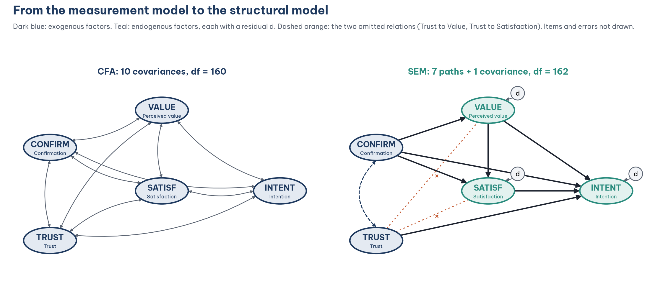
The SEM replaces the 10 factor covariances with 7 hypothesized paths and keeps the covariance between the two exogenous factors, so the degrees of freedom rise from 160 to 162.
With FIML, add a line that fixes the factor means at 0; otherwise JASP 0.99.0 reports 157 degrees of freedom instead of 162.
The structural constraints cost little fit: chi-square rises by 4.38 with 2 degrees of freedom (p = 0.112).
Six of the seven paths are significant; the direct path from confirmation to repurchase intention (H4) is not.
The model explains 33% of the variance in perceived value, 51% in satisfaction and 44% in repurchase intention.
Posts 22 to 25 showed that the measurement model holds up: the five scales fit the data and are reliable, convergent (except the AVE of Repurchase intention) and discriminant. Following the two-step approach (Anderson & Gerbing, 1988), we can now move to the second step: the structural model, where the two-headed arrows between the factors are replaced by directional paths that state the hypotheses.
This post shows how to turn the CFA model into an SEM, run it and read the overall results: model fit, path coefficients and R². Post 27, "Hypothesis Testing in SEM with JASP" goes deeper into testing each hypothesis and interpreting the standardized coefficients.
Sample data and scripts. The data files and scripts for this post are in the research-data-analysis repository on GitHub (folder
data/andscripts/). Download the whole repository with Code > Download ZIP.
About the figures and numbers. The screenshots and result tables come from JASP 0.99.0 (JASP Team, 2026) on macOS, run on the file
marketplace_x_sem.savfrom Post 21, "Preparing and Connecting Data from SPSS to JASP" (267 respondents, missing cells kept). The numbers were checked with the R package lavaan (Rosseel, 2012) in the scriptstructural_model.R(folderscripts/of the repository).
1. From CFA to SEM: what changes?
Exogenous and endogenous variables
An exogenous variable has no arrow pointing at it: CONFIRM and TRUST. The model does not explain them; it only uses them to explain other variables.
An endogenous variable has at least one arrow pointing at it: VALUE, SATISF and INTENT. Each endogenous variable needs a structural residual (d, disturbance): the part of its variance that the variables before it do not explain.
SATISF is both an outcome (of CONFIRM and VALUE) and a cause (of INTENT). Ordinary regression cannot do this in one equation, but SEM estimates all the equations at once (Post 19, "What Is AMOS? CB-SEM and When to Use It Instead of SPSS").
The seven hypotheses
Note on numbering. Posts 2 and 14 use six hypotheses, in which H4 is Perceived value to Repurchase intention, H5 is Satisfaction to Repurchase intention and H6 is Trust to Repurchase intention. From this post on, the model adds a direct path from Confirmation to Repurchase intention (to test the direct effect alongside the indirect paths through Perceived value and Satisfaction, Post 28, "Mediation Analysis with JASP"), so this path takes the number H4 and the next three hypotheses move to H5 (Perceived value), H6 (Satisfaction) and H7 (Trust); H1 to H3 stay the same.
Where do the extra degrees of freedom come from?
The CFA has 10 covariances among the five factors. The SEM replaces them with 7 paths and keeps 1 covariance, between the two exogenous factors CONFIRM and TRUST. The SEM therefore has 2 parameters fewer than the CFA: the two relations that are not hypothesized, TRUST to VALUE and TRUST to SATISF (the dashed orange lines in Figure 1). The degrees of freedom rise from 160 to 162.
Important rule: always let the exogenous variables correlate, unless theory says they are independent (Kline, 2023). AMOS does not draw this covariance for you; forgetting it is a very common mistake (Section 5).
2. Specify the structural model in JASP
The Factor module only runs CFA. The structural model needs the SEM module (switch it on with the plus button at the right end of the toolbar, Post 22):
Open
marketplace_x_sem.savand choose SEM > Structural Equation Modeling.Type the model in the editor in lavaan syntax, then press Cmd+Enter (Figure 2):
# Measurement model
CONFIRM =~ CONF1 + CONF2 + CONF3 + CONF4
VALUE =~ PV1 + PV2 + PV3 + PV4
SATISF =~ SAT1 + SAT2 + SAT3 + SAT4
TRUST =~ TRU1 + TRU2 + TRU3 + TRU4R
INTENT =~ RI1 + RI2 + RI3 + RI4
# Structural model
VALUE ~ CONFIRM
SATISF ~ CONFIRM + VALUE
INTENT ~ CONFIRM + VALUE + SATISF + TRUST
CONFIRM ~~ TRUST
# Fix the factor means at 0 (as in AMOS)
CONFIRM + VALUE + SATISF + TRUST + INTENT ~ 0*1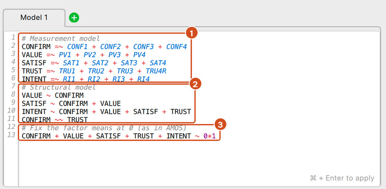
Three operators to remember:
lavaan adds a residual automatically to every endogenous variable, so you do not need to declare d1, d2 and d3. The latent variable names must be spelled exactly as in the measurement part; comment lines start with #.
The last line is required with FIML. As in Post 22, the SEM module of JASP 0.99.0 also estimates the factor means when FIML is used, which makes the degrees of freedom come out wrong (157 instead of 162). Fixing the factor means at 0, as AMOS and the CFA module do, gives the correct degrees of freedom and chi-square.
Check that Missing data handling under Estimation Options is FIML (the default of the SEM module when the data have missing cells; the output notes that "Missing data method 'FIML' forces meanstructure").
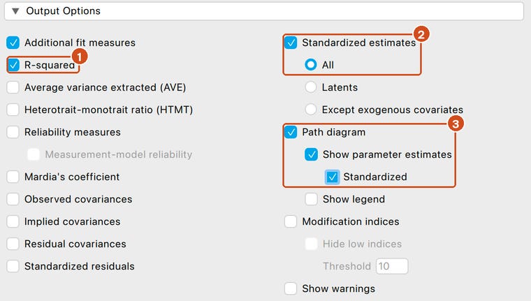
Tick under Output Options (Figure 3): Additional fit measures, R-squared, Standardized estimates (choose All) and Path diagram with Show parameter estimates and Standardized.
3. Read the results
Model fit: SEM compared with CFA
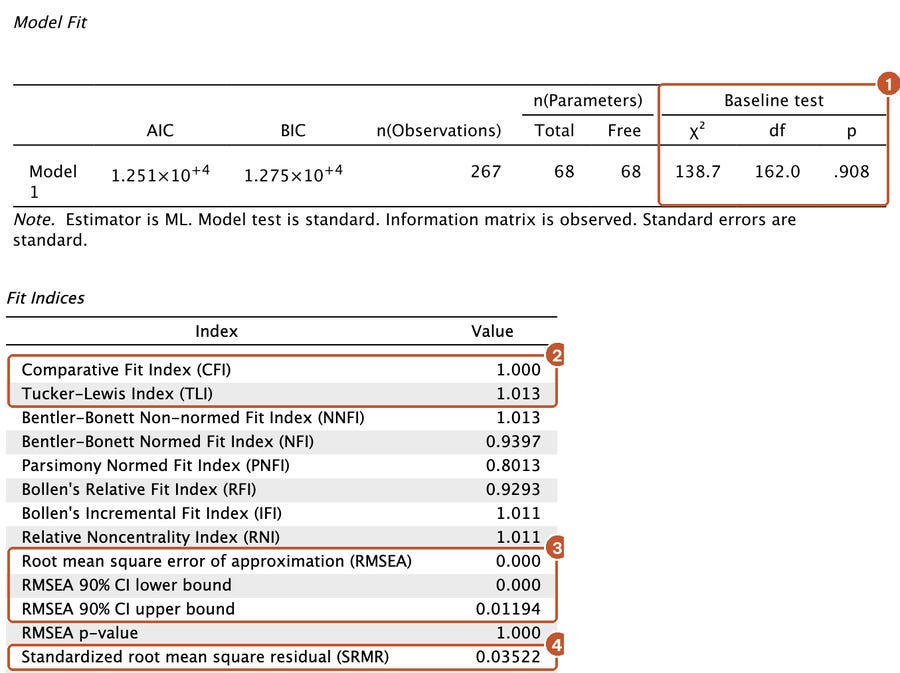
A structural model cannot fit better than the CFA, because it is the CFA with extra constraints (Anderson & Gerbing, 1988). The right question is whether those constraints cost much fit. Comparing the two nested models, the chi-square rises by 4.38 with 2 degrees of freedom, p = 0.112 (computed in lavaan from the unrounded values 134.29 and 138.67). The two omitted relations (Trust to Value and Trust to Satisfaction) are not needed to explain the data. The other indices hardly change.
The standardized loadings in the SEM differ from the CFA by at most 0.002. If the loadings changed noticeably when moving to the SEM, that would signal a misspecified structural model that is "pulling" the measurement model (Kline, 2023).
Path coefficients
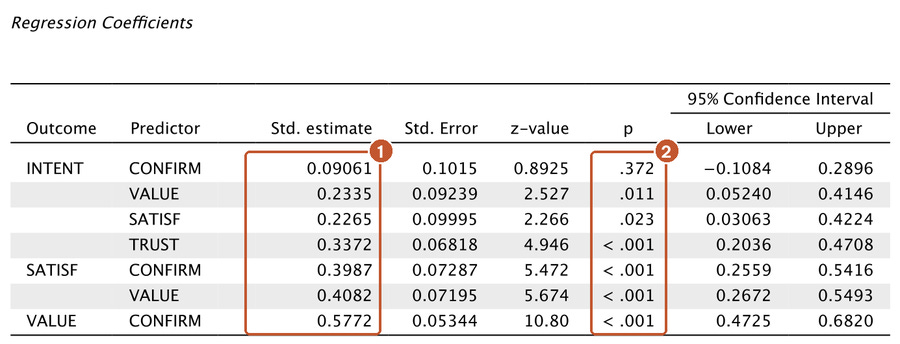
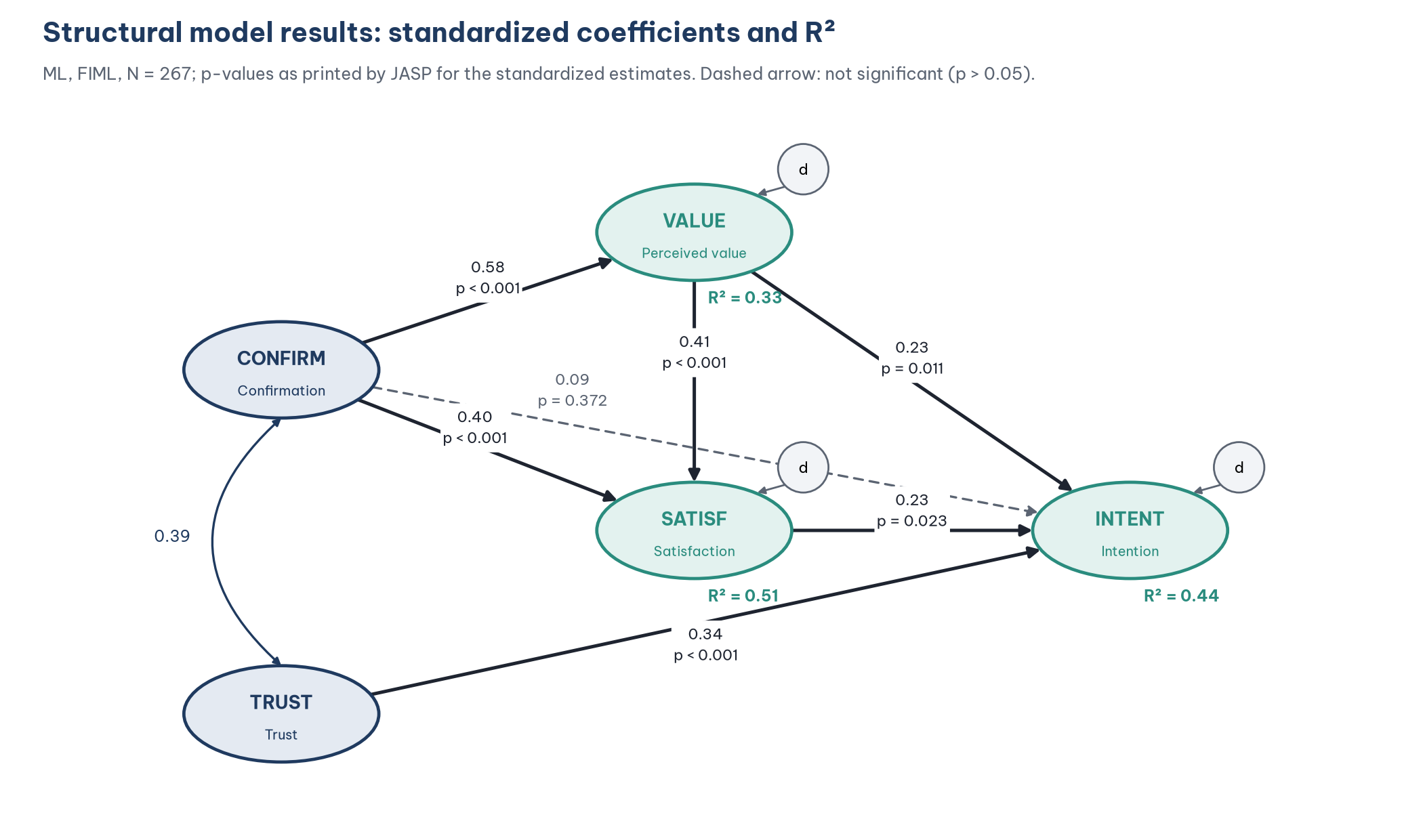
Six of the seven paths are significant at the 0.05 level; H4 is not. With standardization set to All, JASP tests the standardized coefficients, so its z and p differ slightly from the test of the unstandardized coefficients that AMOS reports as C.R. (for example H5: p = 0.011 here, 0.015 for the unstandardized coefficient). The conclusions are the same. This result agrees with the regression on mean scores in Post 14 in direction and significance, but the standardized coefficients in the SEM are larger because measurement error has been removed (Post 19). Post 27 interprets each hypothesis, compares the size of the coefficients and shows how to write the conclusions.
In AMOS. The unstandardized coefficients are under Estimates > Scalars > Regression Weights in the Text Output (the same table as the loadings; the rows look like VALUE <--- CONFIRM), with C.R. as the z-value; the standardized coefficients are under Standardized Regression Weights (Byrne, 2016). With the AMOS settings (ML, FIML, N = 267), the unstandardized estimates, with S.E., C.R. and p, are: H1 0.627 (0.087; 7.22; < 0.001); H2 0.412 (0.085; 4.87; < 0.001); H3 0.389 (0.077; 5.02; < 0.001); H4 0.088 (0.099; 0.89; 0.375); H5 0.208 (0.085; 2.44; 0.015); H6 0.212 (0.095; 2.23; 0.026); H7 0.316 (0.071; 4.46; < 0.001). The standardized coefficients are the same as in the table above.
The covariance between CONFIRM and TRUST corresponds to a correlation of 0.39 (p < 0.001, Factor Covariances table), which confirms that letting the two exogenous factors correlate is necessary.
R² of the endogenous variables
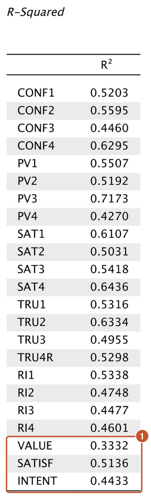
The standardized residual variance equals 1 − R² (for example 0.557 for INTENT, Factor Variances table). The R² of INTENT (0.443) is clearly higher than in the regression of Post 14 (0.315), again because SEM removes measurement error.
The JASP path diagram
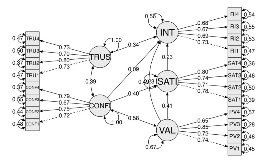
The JASP diagram (drawn with the semPlot package) is good enough to check the specification: the right number of arrows, the right directions and a two-headed arrow between CONFI and TRUS (0.39). For a thesis, redraw it more cleanly, as in Figure 6.
4. Indirect and total effects
With Standardized estimates ticked, JASP also prints the Indirect Effects and Total Effects tables, with standard errors computed by the delta method.
CONFIRM affects INTENT through three indirect paths: via VALUE (0.135, p = 0.014), via SATISF (0.090, p = 0.038) and via VALUE then SATISF (0.053, p = 0.038). The direct effect is small and not significant (0.09), but the total effect is 0.37 (p < 0.001, 95% CI [0.231, 0.508]). This is a sign of mediation: confirmation of expectations affects repurchase intention mainly through perceived value and satisfaction. A rigorous test of indirect effects needs bootstrapping, the topic of Post 28.
5. A common mistake: forgetting the covariance between exogenous variables
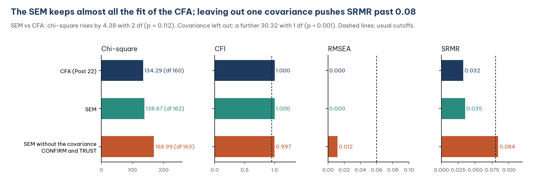
If the two-headed arrow between CONFIRM and TRUST is left out, the model assumes that the two concepts are uncorrelated. On the sample data, the chi-square rises by 30.32 with 1 degree of freedom (p < 0.001) and SRMR rises to 0.084, above the 0.08 cutoff, while CFI (0.997) and RMSEA (0.012) still look excellent. This illustrates the advice in Post 23, "SEM Model Fit Indices in JASP": read several indices. SRMR is sensitive to this kind of error because it measures the gap between correlations directly.
lavaan lets latent exogenous variables correlate by default, so the line CONFIRM ~~ TRUST is in fact redundant in JASP. The post keeps it to make the model explicit and to match the AMOS diagram. AMOS users must draw this arrow themselves.
6. Reporting the results
The structural model fit the data: chi-square = 138.67, df = 162, p = 0.908; CFI = 1.000; TLI = 1.013; RMSEA = 0.000 (90% CI [0.000, 0.012]); SRMR = 0.035. Compared with the measurement model, the structural model did not significantly worsen fit (chi-square difference = 4.38 with 2 degrees of freedom, p = 0.112). The model explained 33.3% of the variance in perceived value, 51.4% in satisfaction and 44.3% in repurchase intention.
The table of path coefficients and the diagram with standardized coefficients are reported together with the conclusion for each hypothesis in Post 27.
Five common mistakes
Running the SEM before evaluating the measurement model. Path coefficients cannot be trusted if the scales do not hold up.
Forgetting the residual of an endogenous variable (AMOS reports an error) or forgetting the covariance between exogenous variables (AMOS reports no error; the model just fits worse).
Adding paths because of modification indices to improve fit without a hypothesis.
Skipping the comparison with the CFA. SEM fit must be read relative to the CFA.
Reporting only the significant coefficients and leaving out rejected hypotheses such as H4.
Frequently asked questions
Should I run SEM on mean scores (path analysis) instead of latent variables?
Path analysis on mean scores is simultaneous regression and still ignores measurement error, as in Post 14. With multi-item scales that have passed a CFA, full SEM is the better choice; path analysis suits samples that are small relative to the number of parameters.
Unstandardized or standardized coefficients?
Report both, or at least the standardized coefficients with p. The significance test that AMOS reports (C.R., p) is based on the unstandardized coefficients. Post 27 discusses this in detail.
How high should R² be?
There is no general cutoff; it depends on the field. In consumer behavior research, an R² of 0.3 to 0.5 for the main outcome is common. Chin (1998) suggests 0.19, 0.33 and 0.67 as weak, moderate and substantial, but these levels were proposed for PLS-SEM.
What about control variables (gender, income)?
Add them as observed exogenous variables, draw arrows to the outcome and let them correlate with the other exogenous variables. For a nominal variable with several groups, use dummy variables (Post 16, "Dummy Variables and Moderator Variables in Regression with PSPP (SPSS)") or multigroup analysis (Post 29, "Multigroup Analysis and Moderation with JASP").
References
Anderson, J. C., & Gerbing, D. W. (1988). Structural equation modeling in practice: A review and recommended two-step approach. Psychological Bulletin, 103(3), 411–423. https://doi.org/10.1037/0033-2909.103.3.411
Byrne, B. M. (2016). Structural equation modeling with AMOS: Basic concepts, applications, and programming (3rd ed.). Routledge.
Chin, W. W. (1998). The partial least squares approach to structural equation modeling. In G. A. Marcoulides (Ed.), Modern methods for business research (pp. 295–336). Lawrence Erlbaum Associates.
JASP Team. (2026). JASP (Version 0.99.0) [Computer software]. https://jasp-stats.org/
Kline, R. B. (2023). Principles and practice of structural equation modeling (5th ed.). Guilford Press.
Rosseel, Y. (2012). lavaan: An R package for structural equation modeling. Journal of Statistical Software, 48(2), 1–36. https://doi.org/10.18637/jss.v048.i02
Discussion about this post