Multigroup Analysis and Moderation in JASP: Invariance and Path Tests
Run a multigroup SEM by gender in free JASP, test measurement invariance, compare each path and test a continuous moderator with product indicators


Key takeaways
Test configural, metric and scalar invariance before comparing paths or latent means; here all three hold.
In JASP 0.99.0, equality constraints on paths take effect only when the syntax contains at least one
:=defined parameter.Constraining the seven paths to be equal does not worsen the fit (p = 0.484): gender does not moderate the model.
A path that is significant for women and not for men is not evidence of moderation; test the difference itself.
Test a continuous moderator with a latent interaction, not a median split; trust does not moderate satisfaction (p = 0.615).
Posts 26 to 28 estimated one model for all respondents. The natural next question is whether that model holds equally for every group of customers. For example, does trust affect the repurchase intention of women more strongly than that of men? That is a question about a moderator.
This post does two things:
Multigroup analysis by gender: test measurement invariance, then compare the seven paths between men and women.
A continuous moderator: test whether trust moderates the effect of satisfaction, using a latent interaction variable.
Both results are not significant. The post keeps them as they are and uses them to show a very common error of interpretation: seeing a coefficient that is significant in one group and not in the other, and concluding that there is moderation.
Sample data and scripts. The data files and scripts for this post are in the research-data-analysis repository on GitHub (folder
data/andscripts/). Download the whole repository with Code > Download ZIP.
About the figures and numbers. The screenshots come from JASP 0.99.0 (JASP Team, 2026) on macOS, and the result tables are taken from JASP's Export Results. The numbers were checked with the lavaan package for R (Rosseel, 2012), using the scripts
multigroup.Randcontinuous_moderation.Rin the repository: both give the same results to the third decimal. Where JASP does not print a number (CFI, RMSEA, SRMR, the two-decimal chi-square differences, R², standardized coefficients of the interaction model), the number comes from lavaan and the text says so.
1. Moderators and two ways to test them
A moderator changes the strength or the direction of the effect between two other variables (Baron & Kenny, 1986). It differs from the mediator of Post 28: a mediator is the route the effect travels along, while a moderator is the condition that makes the effect stronger or weaker.
Do not turn a continuous variable into a grouping variable by splitting it at the median: this loses information, reduces power and can produce spurious results (MacCallum et al., 2002). Section 7 shows this on the real data.
2. The multigroup procedure
Comparing paths between two groups only makes sense when both groups understand the scales in the same way. If women read the item "Marketplace X is trustworthy" differently from men, the path coefficients of the two groups measure two different things. That is why measurement invariance must be tested first (Vandenberg & Lance, 2000; Putnick & Bornstein, 2016).
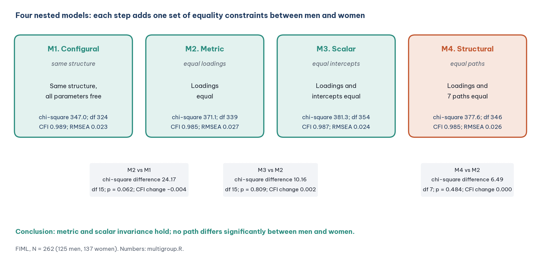
Each step is accepted when the more constrained model does not fit significantly worse. There are two criteria, and it is good practice to report both:
Chi-square difference test: p above 0.05 means the constraints are accepted. This test is sensitive to sample size (Post 23, "SEM Model Fit Indices in JASP").
Change in CFI of no more than −0.01 (Cheung & Rensvold, 2002). Chen (2007) adds: RMSEA should not increase by more than 0.015, and SRMR by no more than 0.030 at the metric step and 0.010 at the scalar step.
The size of each group also matters, because each group has its own set of parameters. The Marketplace X model has 68 free parameters per group in M1; with 125 men and 137 women, that is fewer than 2 respondents per parameter. The model can still be estimated, but the power to detect small differences between the groups is low. Mention this in the limitations.
3. Preparing the data
Five respondents chose "Other" for gender. Five people are not enough to estimate a separate model, so they are left out of the multigroup analysis (not out of the other analyses). The syntax file prepare_post29_data.sps (it runs in SPSS and PSPP; checked in PSPP 2.1.2, Free Software Foundation, 2026) creates these files:
The main part of the syntax:
GET FILE='../data/marketplace_x_sem.sav'.
SELECT IF (GENDER = 1 OR GENDER = 2).
VALUE LABELS GENDER 1 'Male' 2 'Female'.
VARIABLE LEVEL GENDER (NOMINAL).
SAVE OUTFILE='../data/marketplace_x_multigroup.sav'.
The PSPP frequency tables confirm the group sizes: 125 men and 137 women (262) in the first file, and 119 men and 131 women (250) among the respondents who answered all 20 items.
4. Running the multigroup analysis in JASP
Step 1. Open the data and check the grouping variable
Open
marketplace_x_multigroup.savwith the three-line menu button at the top left, then Open > Computer.Check the GENDER column: the icon with three circles (Nominal) and the labels Male and Female (Figure 2, boxes 1 and 2).
Check that the 20 items are Scale (ruler icon, box 3). If they are Ordinal, JASP estimates the model with DWLS instead of ML (Post 20, "Your First Model in JASP").
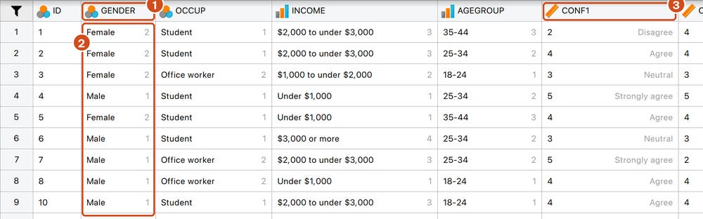
JASP orders the groups by their order of appearance in the data. The first respondent in the file is a woman, so JASP makes Female group 1 and Male group 2. This matters in Steps 4 and 5, when you write labels by group.
Step 2. The configural model (M1)
Choose SEM > Structural Equation Modeling.
Enter the model syntax of Post 26, with a last line that fixes the latent means to 0 (needed with FIML, see Post 26):
CONFIRM =~ CONF1 + CONF2 + CONF3 + CONF4
VALUE   =~ PV1 + PV2 + PV3 + PV4
SATISF  =~ SAT1 + SAT2 + SAT3 + SAT4
TRUST   =~ TRU1 + TRU2 + TRU3 + TRU4R
INTENT  =~ RI1 + RI2 + RI3 + RI4
VALUE   ~ CONFIRM
SATISF  ~ CONFIRM + VALUE
INTENT  ~ CONFIRM + VALUE + SATISF + TRUST
CONFIRM ~~ TRUST
CONFIRM + VALUE + SATISF + TRUST + INTENT ~ 0*1
Check Estimation Options: Missing data handling = (FI)ML (the default).
Open the Multigroup SEM section and set Grouping Variable = GENDER.
Press Cmd + Enter to run the model.
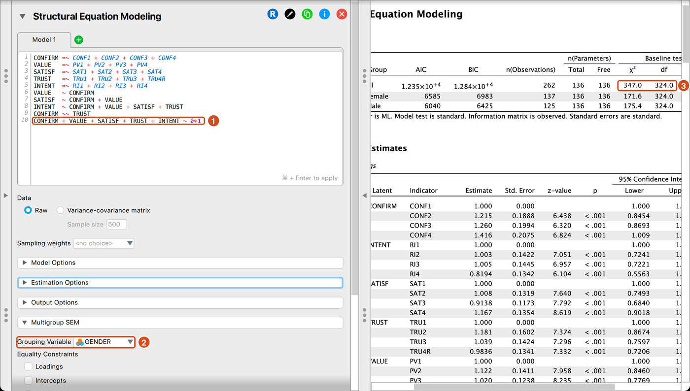
The Model Fit table has three rows: all is the overall result to report; the Female and Male rows are each group's share of the chi-square. Do not use the p column of these two rows for conclusions. The results pane in the screenshots is scrolled slightly to the right, so the first letters of the Group column are cut off.
Step 3. Metric (M2) and scalar (M3) invariance
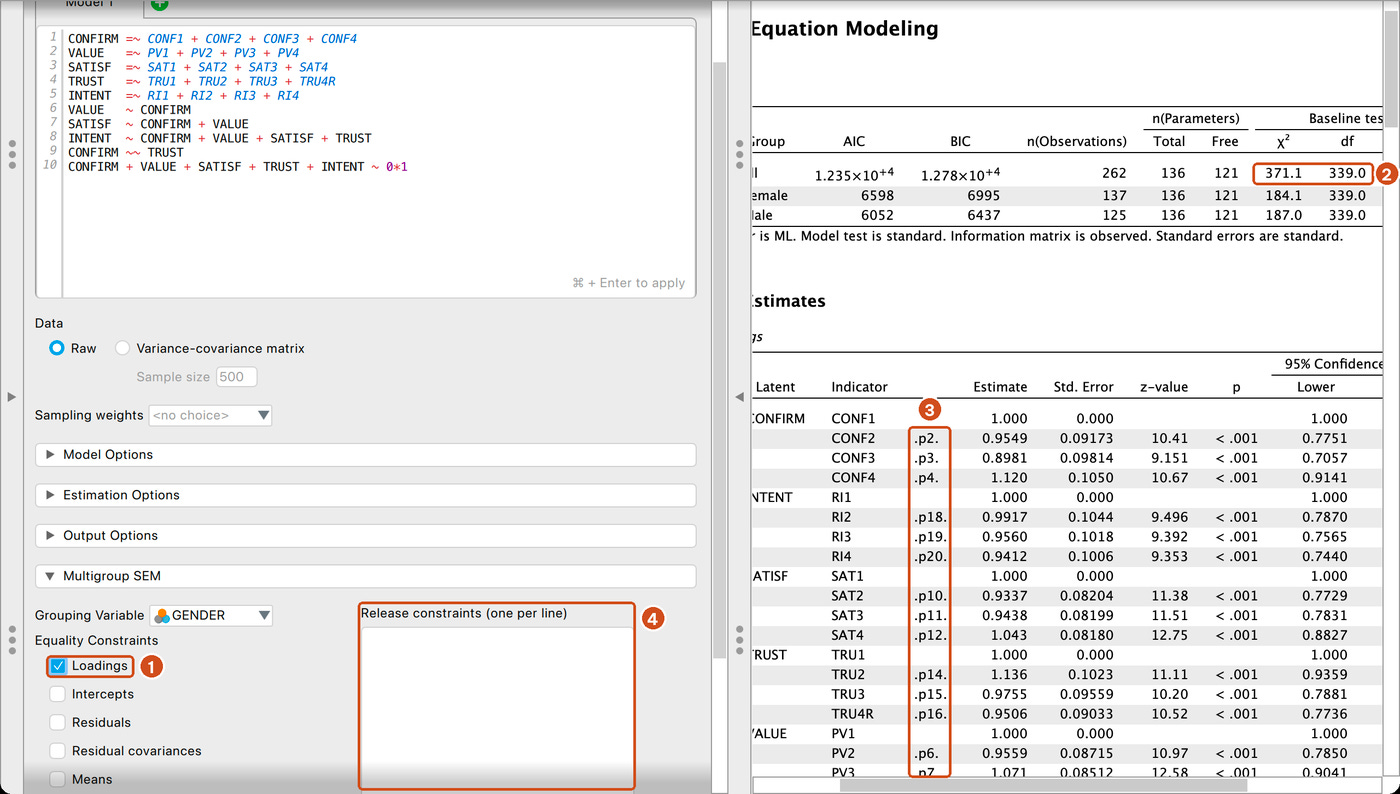
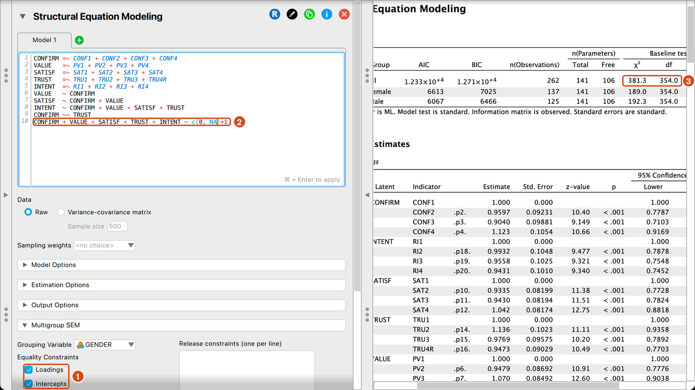
Tick Equality Constraints > Loadings. JASP reruns the model at once (Figure 4).
Write down the chi-square and degrees of freedom: 371.1 and 339.
To test the intercepts:
Tick Intercepts as well.
Change the last line of the syntax to
CONFIRM + VALUE + SATISF + TRUST + INTENT ~ c(0, NA)*1. The 0 fixes the latent means of group 1 (Female, the reference group);NAfrees the means of group 2 (Male). If you keep0*1for both groups, any difference in mean level is pushed into the intercepts and the test is wrong.Press Cmd + Enter.
In AMOS
AMOS fits the same nested models on the 250 complete respondents (marketplace_x_multigroup_complete.sav). Define the groups Male and Female in Analyze > Manage Groups, then link each group to the file in File > Data Files with Grouping Variable GENDER and Group Value 1 (Male) or 2 (Female). Tick Estimate means and intercepts (Estimation tab) and Critical ratios for differences (Output tab) in View > Analysis Properties. Then choose Analyze > Multiple-Group Analysis: AMOS labels every parameter by group and creates the Unconstrained, Measurement weights, Measurement intercepts and Structural weights models in one run. The Model Comparison section of the Text Output prints the chi-square differences. In AMOS, Male is group 1 and the reference group whose latent means are fixed to 0. With complete cases the conclusions are the same as below: metric 23.82 (15 df), p = 0.068; scalar 12.05 (15 df), p = 0.675; seven equal paths (run again without means) 7.13 (7 df), p = 0.415.
5. Results of the measurement invariance tests
The JASP Model Fit table shows only the chi-square; CFI, RMSEA and SRMR are added by ticking Additional fit measures in Output Options (Post 20). The difference test can be computed by hand: 371.13 − 346.97 = 24.17 with 339 − 324 = 15 degrees of freedom; the p-value comes from =CHISQ.DIST.RT(24.17, 15) in Excel.
Reading the results:
The configural model fits well (CFI 0.989, RMSEA 0.023): both groups have the same five-factor structure.
Metric invariance holds, but it is borderline by the chi-square test: p = 0.062 (FIML) and 0.068 (complete cases). The CFI change is only −0.004, well inside the 0.01 threshold. SRMR increases by 0.010, below Chen's (2007) 0.030 threshold.
Scalar invariance holds clearly (p = 0.809; CFI does not drop).
A score test on M2 (in lavaan) shows which item deviates most: the loading of PV2 (1-df chi-square = 5.78, p = 0.016). With 15 loadings tested at the same time, a p-value of about 0.016 can easily occur by chance (the Bonferroni threshold is 0.05/15 = 0.003), and the overall test does not reject invariance. So this post does not free the constraint on PV2. If the overall test had been rejected, the remedy would be partial invariance: free the constraints of the one or two items that deviate most, as long as each factor keeps at least two constrained items (Byrne, 2016).
Once scalar invariance holds, the latent means of the two groups can be compared. The Intercepts table of model M3 (Figure 6) gives the means of the Male group relative to the Female group (fixed to 0):
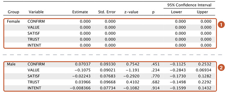
Latent means. No construct has a different mean for men and women: the largest difference is perceived value, where men score 0.11 lower than women (p = 0.234); repurchase intention is almost identical (difference 0.01; p = 0.914). This conclusion is valid only because scalar invariance holds. Comparing mean scores between two groups without testing invariance (for example, a t-test on the average scores, Post 17, "T-Tests in PSPP (SPSS)") silently assumes it.
6. Comparing the paths between men and women
A JASP 0.99.0 pitfall to know about
The obvious way is to untick Intercepts, restore the ~ 0*1 line and tick Equality Constraints > Regressions. When you try this, the chi-square does not change (still 371.1 with 339 degrees of freedom), which means the constraint was not applied. Putting shared labels in the syntax, such as c(h1, h1)*CONFIRM, gives exactly the same result.
The cause: to compute the Indirect Effects and Total Effects tables, JASP gives each path in each group its own label, which overrides the user's constraints. JASP skips this step only when the syntax contains at least one defined parameter with :=. So the correct way is: put the labels in the syntax and add at least one := line. The Regression Coefficients table of model M2 (Figure 7) shows what JASP prints without such a line: no labels, and a separate coefficient for each group.
Way 1. Constrain all seven paths at once (M4)
Untick Intercepts and keep Loadings.
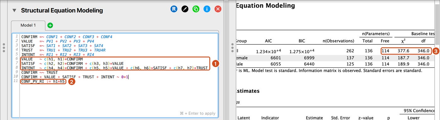
Edit the syntax: give the same label to both groups and add one defined parameter. The indirect effect
CONF_PV_RI(CONFIRM to VALUE to INTENT) was chosen because it is meaningful for the study (Post 28), not only to work around the pitfall:
VALUE   ~ c(h1, h1)*CONFIRM
SATISF  ~ c(h2, h2)*CONFIRM + c(h3, h3)*VALUE
INTENT  ~ c(h4, h4)*CONFIRM + c(h5, h5)*VALUE + c(h6, h6)*SATISF + c(h7, h7)*TRUST
CONFIRM ~~ TRUST
CONFIRM + VALUE + SATISF + TRUST + INTENT ~ 0*1
CONF_PV_RI := h1*h5
Press Cmd + Enter. The number of free parameters drops from 121 to 114 and the degrees of freedom rise from 339 to 346: the constraints are now in effect.
In M4, both groups now show the same coefficient for each path, and the Defined Parameters table gives CONF_PV_RI = 0.132 (p = .017).
Constraining the seven paths to be equal does not make the model worse. Overall, gender does not moderate the model.
Way 2. Test each path separately
An overall test can hide a difference in one path. To test each path, give each group its own label and define the differences. Remember that group 1 is Female and group 2 is Male:
VALUE   ~ c(h1f, h1m)*CONFIRM
SATISF  ~ c(h2f, h2m)*CONFIRM + c(h3f, h3m)*VALUE
INTENT  ~ c(h4f, h4m)*CONFIRM + c(h5f, h5m)*VALUE + c(h6f, h6m)*SATISF + c(h7f, h7m)*TRUST
CONFIRM ~~ TRUST
CONFIRM + VALUE + SATISF + TRUST + INTENT ~ 0*1
diff_H1 := h1m - h1f
diff_H2 := h2m - h2f
diff_H3 := h3m - h3f
diff_H4 := h4m - h4f
diff_H5 := h5m - h5f
diff_H6 := h6m - h6f
diff_H7 := h7m - h7f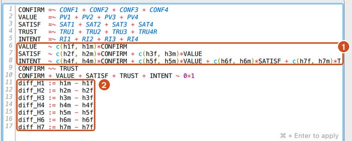
The chi-square is still 371.1 (model M2), because no constraint was added. The Defined Parameters table gives a z test for each difference (Figure 10). This is the equivalent of AMOS's Critical ratios for differences.

An interpretation error to avoid
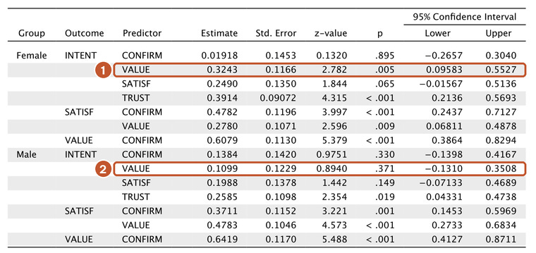
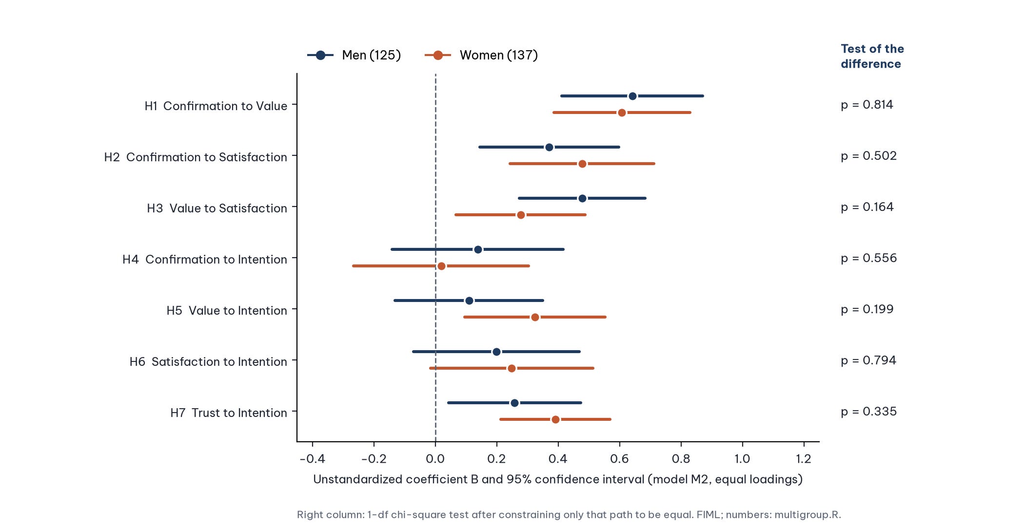
Look at H5: the coefficient is significant for women (p < 0.01) but not significant for men (p close to 0.4). It is very tempting to write "perceived value affects the repurchase intention of women only; gender moderates this relationship". That conclusion is wrong. The direct test of the difference gives a p of about 0.2: the two coefficients are not significantly different. The confidence intervals of the two groups in Figure 11 overlap almost completely.
The difference between "significant" and "not significant" is not itself statistically significant (Gelman & Stern, 2006). A coefficient of 0.32 with p = 0.005 and one of 0.11 with p = 0.37 can easily come from the same true value and differ only through sampling error. A conclusion about moderation must rest on a test of the difference, not on a comparison of two p-values.
A note on power: with about 125 people per group, the standard error of the H5 difference is about 0.17. The true difference would have to be about 0.47 for the test to have 80% power. The "no difference" result here should be written as no difference was detected, not "the two groups are proved to be the same".
7. A continuous moderator: the latent interaction
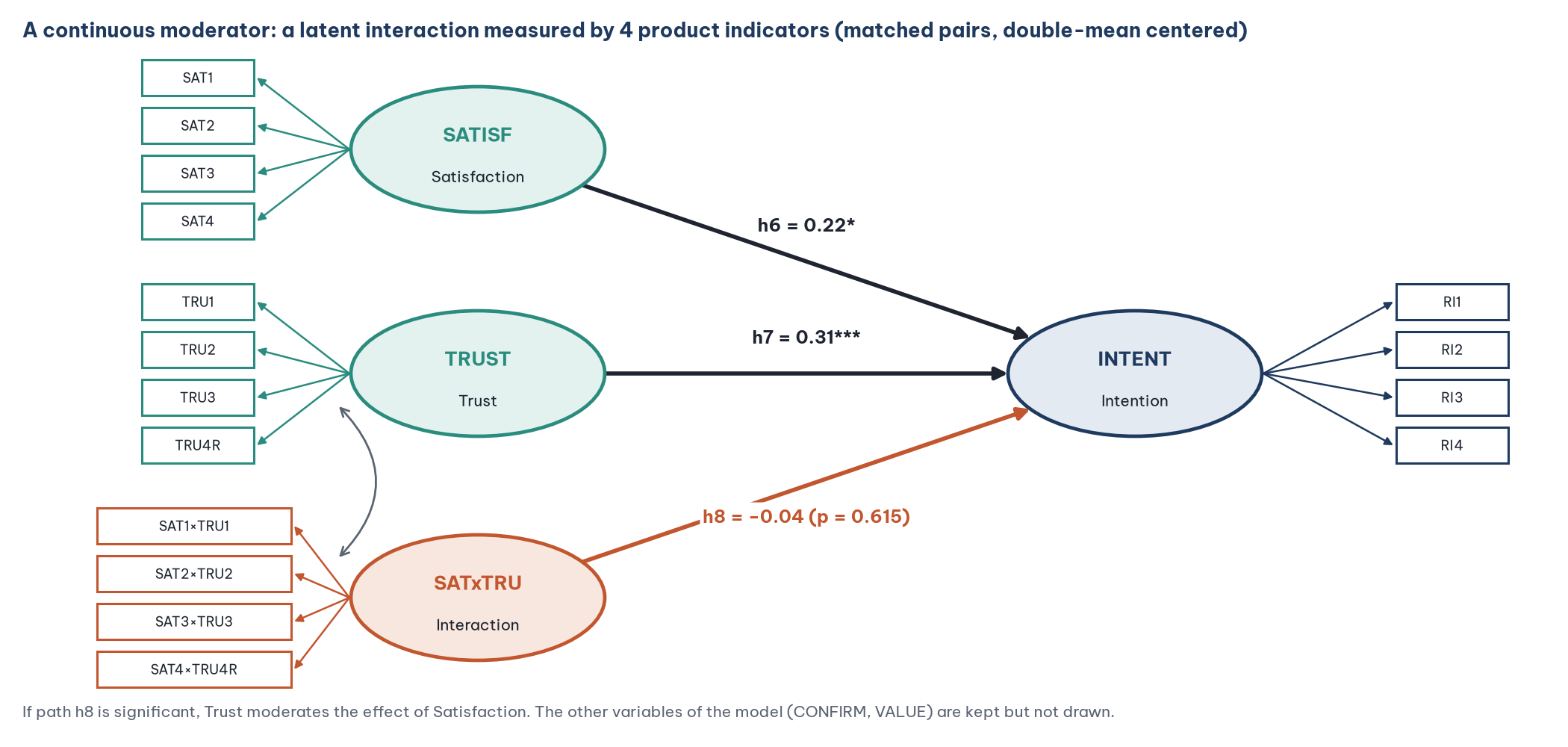
An additional hypothesis: the higher the trust, the weaker the effect of satisfaction on repurchase intention, because customers who trust the marketplace already have a reason to come back even when this purchase was not fully satisfying. It is tested with the product SATISF × TRUST.
In CB-SEM, the product of two latent variables cannot be observed. There are three main approaches (Marsh et al., 2004):
This post uses matched-pair product indicators with double-mean centering (Marsh et al., 2004; Lin et al., 2010), because it works in both AMOS and JASP:
Pair the items: SAT1 with TRU1, SAT2 with TRU2, SAT3 with TRU3, SAT4 with TRU4R. Each item is used only once, so the 4 product indicators have no correlated errors.
Center each item: subtract the item's mean.
Multiply the pairs.
Center again: subtract the mean of each product. This avoids having to estimate an extra, complicated mean structure (Lin et al., 2010).
Part B of prepare_post29_data.sps performs these four steps with AGGREGATE and COMPUTE and saves marketplace_x_product.sav with the variables SATxTRU1 to SATxTRU4. The product indicators equal those of the indProd() function in the semTools package (Jorgensen et al., 2022) to the 15th decimal.
Steps in JASP
Open
marketplace_x_product.sav. Check that SATxTRU1 to SATxTRU4 are Scale.Open a new Structural Equation Modeling analysis (without a grouping variable).
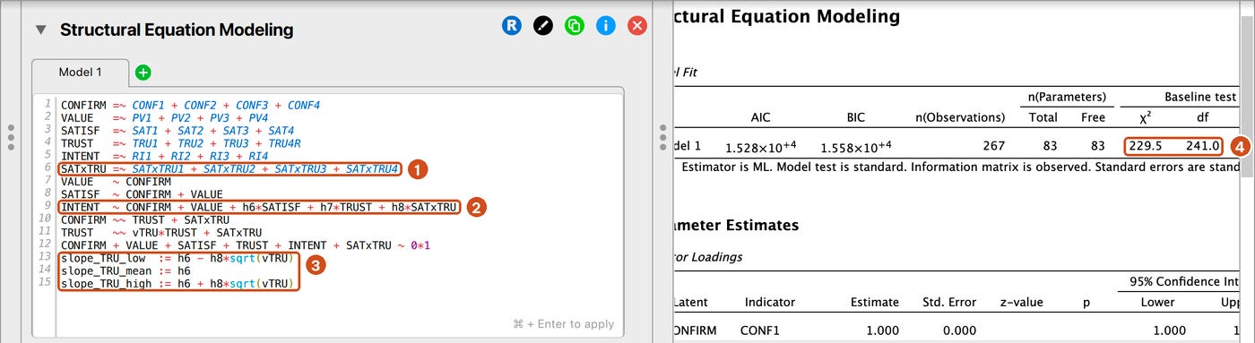
Enter the syntax:
CONFIRM =~ CONF1 + CONF2 + CONF3 + CONF4
VALUE   =~ PV1 + PV2 + PV3 + PV4
SATISF  =~ SAT1 + SAT2 + SAT3 + SAT4
TRUST   =~ TRU1 + TRU2 + TRU3 + TRU4R
INTENT  =~ RI1 + RI2 + RI3 + RI4
SATxTRU =~ SATxTRU1 + SATxTRU2 + SATxTRU3 + SATxTRU4
VALUE   ~ CONFIRM
SATISF  ~ CONFIRM + VALUE
INTENT  ~ CONFIRM + VALUE + h6*SATISF + h7*TRUST + h8*SATxTRU
CONFIRM ~~ TRUST + SATxTRU
TRUST   ~~ vTRU*TRUST + SATxTRU
CONFIRM + VALUE + SATISF + TRUST + INTENT + SATxTRU ~ 0*1
slope_TRU_low  := h6 - h8*sqrt(vTRU)
slope_TRU_mean := h6
slope_TRU_high := h6 + h8*sqrt(vTRU)
The label vTRU is attached to the variance of TRUST so that the simple slopes of SATISF can be computed at low trust (mean minus 1 standard deviation), average trust and high trust (plus 1 standard deviation). The three := lines also make JASP keep the labels h6, h7 and h8 (Section 6).


Results (FIML, N = 267)
In AMOS, the same model is drawn on the 254 complete respondents (marketplace_x_product_complete.sav), with SATxTRU1 to SATxTRU4 as the indicators of a latent variable SATxTRU. The interaction coefficient is h8 = −0.055 (SE 0.082, p = 0.504; beta = −0.050), so the conclusion is the same.
Reading the results:
The interaction coefficient h8 is negative (in the hypothesized direction) but very small and not significant (p = 0.615; the confidence interval contains 0). The R² of repurchase intention rises only from 0.444 to 0.445 when the interaction is added (f² = 0.0003; lavaan). Trust does not moderate the effect of satisfaction.
h6 is now the effect of satisfaction when trust is at its mean, no longer the "overall effect" of Post 26. This is the correct way to read the main coefficient when an interaction is in the model.
Ignore the fit indices of a model with product indicators: the product of two variables is not normally distributed, so the ML chi-square is no longer accurate. The purpose of this model is to test h8.
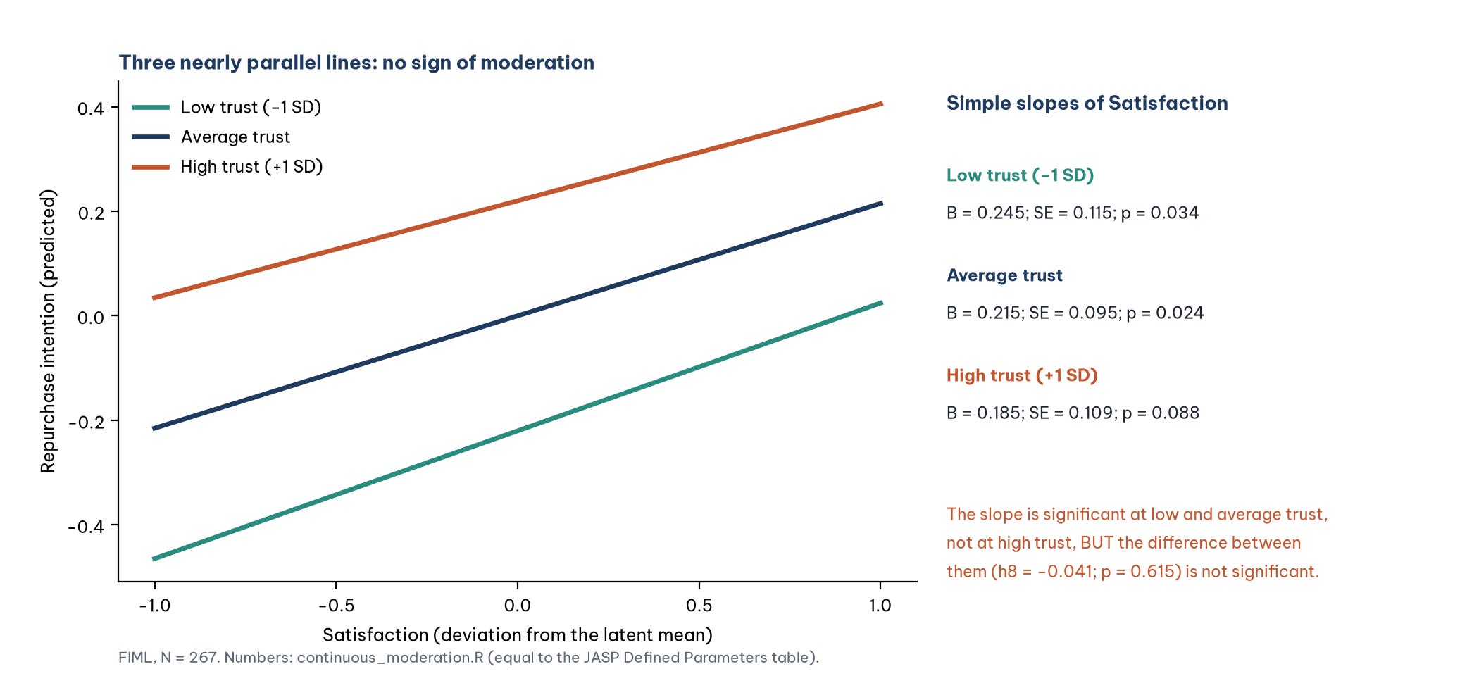
Figure 16 repeats the lesson of Section 6 in another form: the slope of satisfaction is significant at low trust (p = 0.034) and average trust (p = 0.024), and not significant at high trust (p = 0.088). But the three slopes (0.245, 0.215, 0.185) are almost equal and the three lines are nearly parallel. The test of moderation is the test of h8, not a count of which slopes pass the 0.05 threshold.
Trying a median split. If customers are split into a low-trust group (mean TRU score of 4 or less, 151 people) and a high-trust group (above 4, 116 people) and a multigroup model is run, the effect of satisfaction is 0.279 (p = 0.035) in the low group and 0.205 (p = 0.234) in the high group. Again a "significant, not significant" pair, but the difference is not significant (chi-square difference 0.12; p = 0.733; lavaan). The split also creates groups of unequal size, because many people score exactly 4 (the median), and it puts a person scoring 3.75 in the same group as a person scoring 1 (MacCallum et al., 2002).
8. Reporting the results
A multigroup analysis by gender was run with FIML estimation on 262 respondents (125 men, 137 women; 5 respondents who chose another gender were excluded because the group was too small). The configural model fitted well (chi-square = 346.97; df = 324; CFI = 0.989; RMSEA = 0.023). Constraining the loadings to be equal did not significantly worsen the fit (chi-square difference = 24.17; df = 15; p = 0.062; CFI change = −0.004), nor did additionally constraining the intercepts (chi-square difference = 10.16; df = 15; p = 0.809; CFI change = +0.002), indicating metric and scalar invariance across genders (Cheung & Rensvold, 2002). Constraining the seven path coefficients to be equal did not worsen the fit (chi-square difference = 6.49; df = 7; p = 0.484), and no coefficient differed significantly between the groups when tested separately (p from 0.164 to 0.814). Gender did not moderate the relationships in the model. The latent interaction between satisfaction and trust, measured by four matched-pair, double-mean-centered product indicators (Lin et al., 2010), had no significant effect on repurchase intention (B = −0.041; 95% CI [−0.202, 0.119]). With about 130 respondents per group, the power to detect small differences between the groups was limited.
Five common mistakes
Comparing the p-values of two groups instead of testing the difference: concluding "there is moderation" because a coefficient is significant in one group and not in the other.
Skipping measurement invariance and comparing paths or mean scores straight away.
Using only the chi-square difference with a large sample: even tiny differences become significant. Report the changes in CFI, RMSEA and SRMR as well.
Splitting a continuous variable at the median to run a multigroup analysis.
Writing "the two groups are the same" when the test is not significant with small groups. Write "no difference was detected" and mention the limited power.
Frequently asked questions
How many respondents does each group need?
There is no fixed number. Each group must be able to estimate the model on its own (the configural model), so the sample size rules of Post 19, "What Is AMOS? CB-SEM and When to Use It Instead of SPSS" apply to each group. About 100 to 150 respondents per group is a common minimum for a model the size of the Marketplace X model; detecting a path difference of about 0.2 needs considerably more.
What if metric invariance does not hold?
Use a score test (JASP: Modification indices in model M2; AMOS: Modification Indices with a low threshold) to find the item that deviates most, free its constraint (Release constraints in JASP, a separate label in AMOS) and test again. Report clearly which item was freed and why.
Can more than two groups be compared?
Yes, for example four income groups. The procedure is the same; the overall test has more degrees of freedom. When the overall test is significant, compare the groups in pairs and correct for multiple comparisons.
How does SmartPLS handle multigroup analysis?
SmartPLS uses MICOM to test invariance and PLS-MGA or a permutation test to compare paths, and it offers more ways to build interaction terms (Post 41, "Moderation Analysis in SmartPLS 4").
References
Baron, R. M., & Kenny, D. A. (1986). The moderator–mediator variable distinction in social psychological research: Conceptual, strategic, and statistical considerations. Journal of Personality and Social Psychology, 51(6), 1173–1182. https://doi.org/10.1037/0022-3514.51.6.1173
Byrne, B. M. (2016). Structural equation modeling with AMOS: Basic concepts, applications, and programming (3rd ed.). Routledge.
Chen, F. F. (2007). Sensitivity of goodness of fit indexes to lack of measurement invariance. Structural Equation Modeling, 14(3), 464–504. https://doi.org/10.1080/10705510701301834
Cheung, G. W., & Rensvold, R. B. (2002). Evaluating goodness-of-fit indexes for testing measurement invariance. Structural Equation Modeling, 9(2), 233–255. https://doi.org/10.1207/S15328007SEM0902_5
Free Software Foundation. (2026). GNU PSPP (Version 2.1.2) [Computer software]. https://www.gnu.org/software/pspp/
Gelman, A., & Stern, H. (2006). The difference between "significant" and "not significant" is not itself statistically significant. The American Statistician, 60(4), 328–331. https://doi.org/10.1198/000313006X152649
JASP Team. (2026). JASP (Version 0.99.0) [Computer software]. https://jasp-stats.org/
Jorgensen, T. D., Pornprasertmanit, S., Schoemann, A. M., & Rosseel, Y. (2022). semTools: Useful tools for structural equation modeling (R package version 0.5-6) [Computer software]. https://CRAN.R-project.org/package=semTools
Lin, G.-C., Wen, Z., Marsh, H. W., & Lin, H.-S. (2010). Structural equation models of latent interactions: Clarification of orthogonalizing and double-mean-centering strategies. Structural Equation Modeling, 17(3), 374–391. https://doi.org/10.1080/10705511.2010.488999
MacCallum, R. C., Zhang, S., Preacher, K. J., & Rucker, D. D. (2002). On the practice of dichotomization of quantitative variables. Psychological Methods, 7(1), 19–40. https://doi.org/10.1037/1082-989X.7.1.19
Marsh, H. W., Wen, Z., & Hau, K.-T. (2004). Structural equation models of latent interactions: Evaluation of alternative estimation strategies and indicator construction. Psychological Methods, 9(3), 275–300. https://doi.org/10.1037/1082-989X.9.3.275
Putnick, D. L., & Bornstein, M. H. (2016). Measurement invariance conventions and reporting: The state of the art and future directions for psychological research. Developmental Review, 41, 71–90. https://doi.org/10.1016/j.dr.2016.06.004
Rosseel, Y. (2012). lavaan: An R package for structural equation modeling. Journal of Statistical Software, 48(2), 1–36. https://doi.org/10.18637/jss.v048.i02
Vandenberg, R. J., & Lance, C. E. (2000). A review and synthesis of the measurement invariance literature: Suggestions, practices, and recommendations for organizational research. Organizational Research Methods, 3(1), 4–70. https://doi.org/10.1177/109442810031002
Discussion about this post