Hypothesis Testing in SEM with JASP: Coefficients, p-Values and f²
Label the paths in free JASP, read standardized coefficients, p-values and confidence intervals, compare two coefficients and compute f² for every hypothesis


Key takeaways
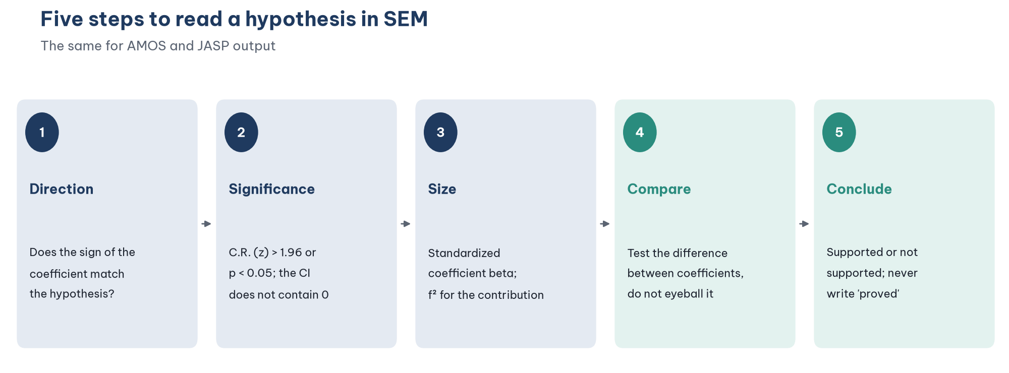
Read each hypothesis in five steps: direction, significance, size, comparison and conclusion.
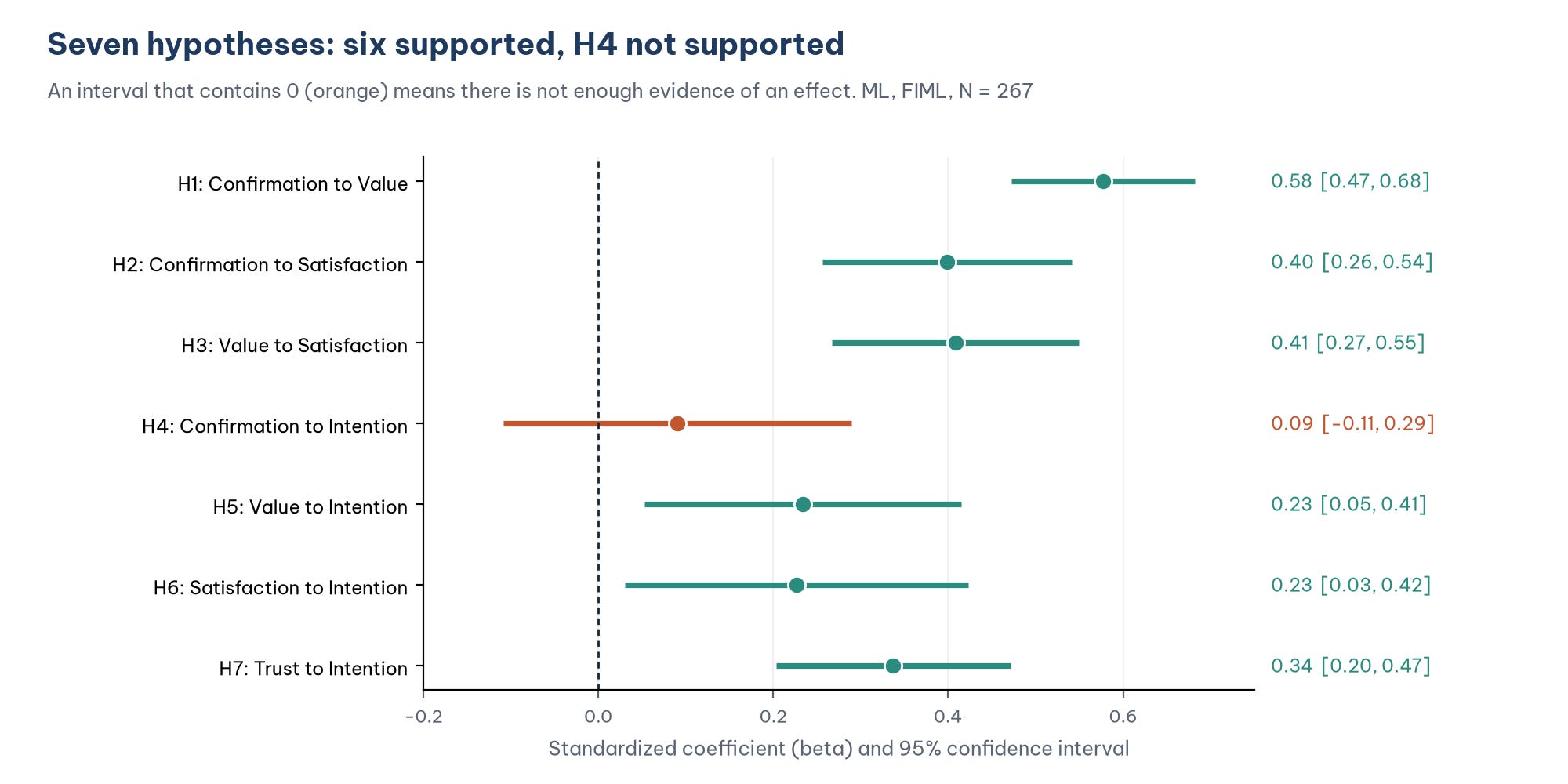
Six of the seven hypotheses are supported; H4 (beta = 0.09, p = 0.372) means no evidence of a direct effect, not "no effect".
State whether a p-value tests B or beta: JASP with Standardized estimates = All tests beta and AMOS tests B; the two differ slightly.
f² measures the unique contribution of a direct path: VALUE is significant (beta = 0.23) yet its f² is only 0.012.
Do not rank coefficients by eye: trust (0.34) and satisfaction (0.23) do not differ significantly (p = 0.379).
Post 26, "Structural Equation Model (SEM) in JASP" ran the structural model and found that six of the seven paths were significant. This post goes deeper into the question that the results chapter of every thesis has to answer: is each hypothesis supported or not, and how strong is the effect? It shows how to read unstandardized and standardized coefficients, p-values and confidence intervals correctly, how to measure effect size with f², how to compare two coefficients with a test instead of by eye and how to write the conclusion for a hypothesis that is not supported.
Sample data and scripts. The data files and scripts for this post are in the research-data-analysis repository on GitHub (folder
data/andscripts/). Download the whole repository with Code > Download ZIP.
About the figures and numbers. The screenshots come from JASP 0.99.0 (JASP Team, 2026) on macOS, continuing the SEM analysis of Post 26 on the data file
marketplace_x_sem.sav. The result tables are taken from JASP's Export Results. The numbers were checked with the lavaan package for R (Rosseel, 2012), using the scripthypothesis_testing.Rin the repository.
1. Unstandardized and standardized coefficients
Each path has two coefficients:
Unstandardized coefficient (B): when the cause increases by one unit, the outcome changes by B units, holding the other variables constant. A latent variable takes the unit of the item whose loading is fixed to 1 (Post 20, "Your First Model in JASP"), so B is hard to interpret directly. Significance tests (S.E., C.R., p) are computed on B.
Standardized coefficient (beta): when the cause increases by one standard deviation, the outcome changes by beta standard deviations. Beta is used to compare the size of paths within the same model.
Kline (2023) recommends reporting both, or at least beta together with p.
2. Label the paths and read the output in JASP
Open the SEM analysis of Post 26 and edit the structural part of the model to add labels h1 to h7 in front of the names of the causes (Figure 2):
VALUE ~ h1*CONFIRM
SATISF ~ h2*CONFIRM + h3*VALUE
INTENT ~ h4*CONFIRM + h5*VALUE + h6*SATISF + h7*TRUST
CONFIRM ~~ TRUST
CONFIRM + VALUE + SATISF + TRUST + INTENT ~ 0*1
# Compare two coefficients: Trust and Satisfaction to Intention
diff_TRU_SAT := h7 - h6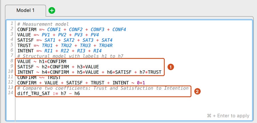
Labels do not change the results; they only give the parameters names so that you can reuse them. A := line defines a new parameter computed from labeled parameters; JASP prints it in the Defined Parameters table. Press Cmd + Enter to apply the syntax.
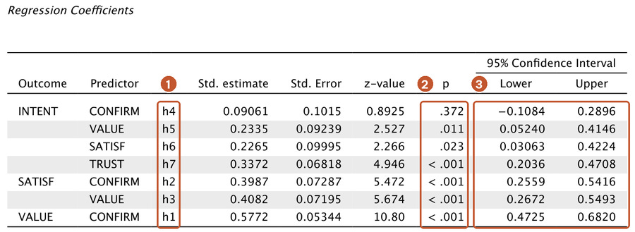
With Standardized estimates ticked and All selected in Output Options, the Std. estimate column is beta, and the standard error, z-value, p and confidence interval refer to beta. JASP lists the outcomes in the order INTENT, SATISF, VALUE, so read the labels rather than the row order. Untick Standardized estimates to see B with its own standard error, z-value (the equivalent of AMOS's C.R.), p and confidence interval. The test of beta and the test of B give slightly different p-values: lavaan's test of B, which AMOS also reports, gives 0.375 for h4, 0.015 for h5 and 0.026 for h6, against .372, .011 and .023 in Figure 3. The conclusions are the same. This post reports the numbers JASP prints with Standardized estimates = All.
For bootstrap confidence intervals, set Standard errors to Bootstrap in Estimation Options and enter the number of Bootstrap samples (Post 28, "Mediation Analysis with JASP" uses 2000, Type Percentile, random seed 2026). With 267 respondents and FIML, each run takes a few minutes.
In AMOS, the same output is in View > Text Output (F10) > Estimates: the Regression Weights table gives B, S.E., C.R. (B divided by S.E.) and P, and Standardized Regression Weights gives beta. For H1 to H7, B = 0.627, 0.412, 0.389, 0.088, 0.208, 0.212 and 0.316, with C.R. = 7.22, 4.87, 5.02, 0.89, 2.44, 2.23 and 4.46. The P column prints three asterisks (***) when p < 0.001; report it as "p < 0.001". AMOS prints confidence intervals only after a bootstrap (Analysis Properties > Bootstrap), which needs the complete-case file marketplace_x_sem_complete.sav. To label a path, double-click the arrow and type the label in the Regression weight box of Object Properties, or label every parameter with Plugins > Name Parameters.
3. Results for the seven hypotheses
Read each hypothesis with the five steps of Figure 1, for example H7:
Read the direction. beta = 0.34 is positive, in the hypothesized direction (higher trust goes with higher repurchase intention).
Read the significance. z = 4.95 > 1.96; p < 0.001; the confidence interval [0.20, 0.47] does not contain 0.
Read the size. When trust increases by one standard deviation, repurchase intention increases by 0.34 standard deviations, holding the other three variables constant.
Compare. It is the largest coefficient among the four predictors of intention, but it is not necessarily significantly larger (Section 6).
Conclude. H7 is supported.
Interpreting H4, which is not supported
H4 has p = 0.372 and its confidence interval contains 0. The correct wording is: "there is no evidence of a direct effect of expectation confirmation on repurchase intention once perceived value, satisfaction and trust are taken into account". Do not write "expectation confirmation does not affect repurchase intention", because:
A non-significant result does not prove that the effect is zero (Post 17, "T-Tests in PSPP (SPSS)"). The confidence interval shows that the true effect could lie anywhere from −0.11 to 0.29.
Expectation confirmation still has a substantial total effect (0.37) through perceived value and satisfaction (Post 26). This result suggests full mediation, which Post 28 tests.
The sample data were simulated with a direct effect of zero (Post 19, "What Is AMOS? CB-SEM and When to Use It Instead of SPSS"), so not supporting H4 here matches the truth of the simulated population.
4. Confidence intervals and bootstrapping
The p-values and confidence intervals above rely on the assumption that the estimates are normally distributed. Bootstrapping does not need this assumption: it draws 2000 samples with replacement from the data, re-estimates the model each time and takes the 2.5th and 97.5th percentiles of the coefficients as the confidence interval (Kline, 2023).
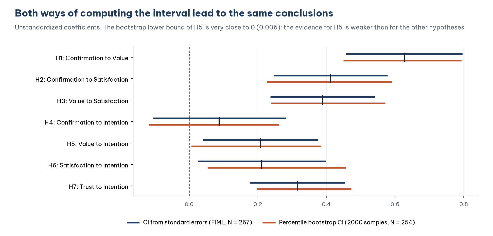
Both methods lead to the same conclusion for all seven hypotheses. The bootstrap lower bound of H5 is only 0.006, very close to 0: the evidence for the effect of perceived value on repurchase intention is weaker than for the other hypotheses, and the conclusion could change in another sample. This is worth reporting, and the p-value of 0.011 alone does not show it.
Bootstrapping is especially advisable when the data are non-normal (Mardia's coefficient above 5, Post 22, "Confirmatory Factor Analysis (CFA) in JASP") or when testing indirect effects (Post 28).
5. Effect size: f²
Beta tells you the size of each path, but it does not directly tell you how much each variable contributes to R². The f² effect size (Cohen, 1988) measures how much R² drops when one path is removed:
f² = (full R² − R² without the path) / (1 − full R²)
Cohen's thresholds: 0.02 is small, 0.15 is medium and 0.35 is large. Remove one path to INTENT at a time, rerun the model and record the R² of INTENT:
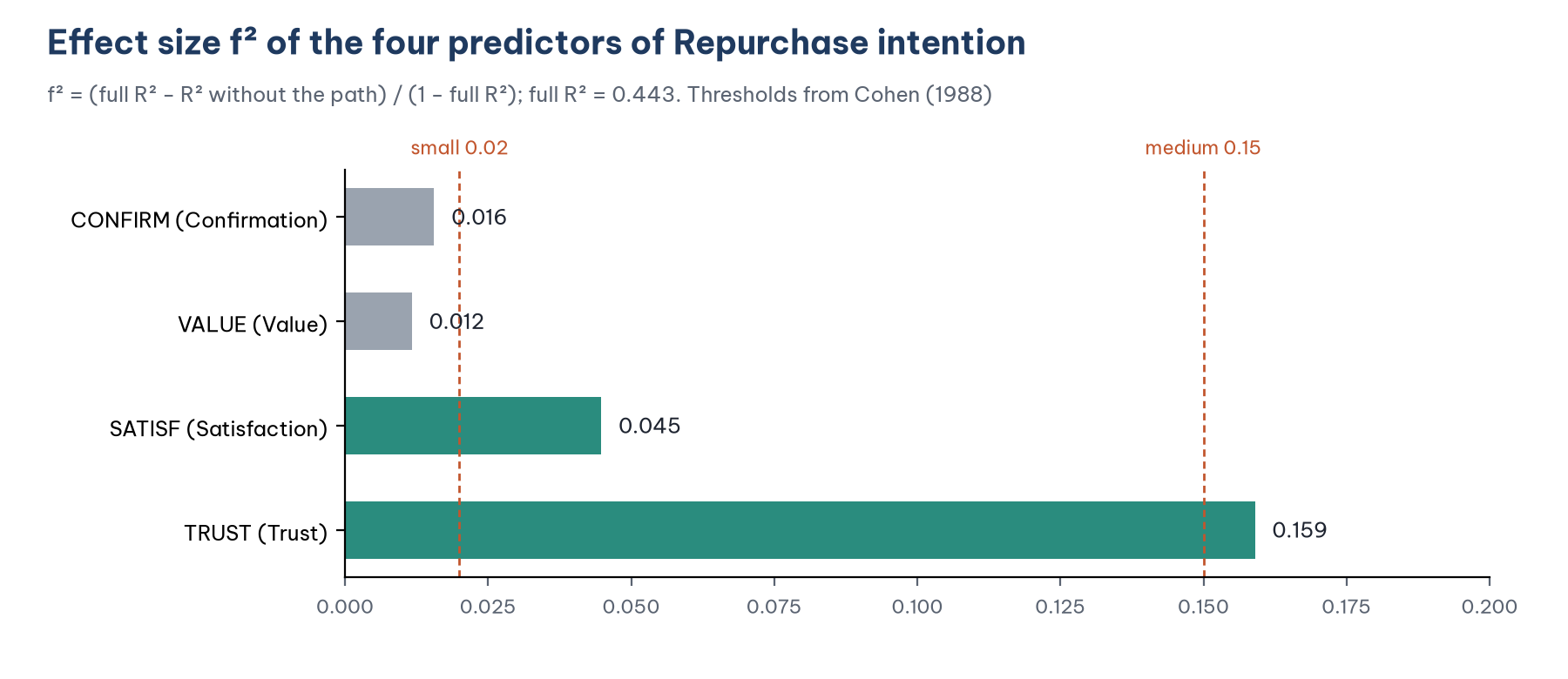
A notable result: VALUE has beta = 0.23 and is significant, yet its f² is only 0.012. The reason is that when the direct path from VALUE to INTENT is removed, most of VALUE's effect still flows through SATISF (VALUE affects SATISF with beta = 0.41), so the R² of INTENT barely drops. f² measures the unique contribution of the direct path, not the overall importance of the variable.
f² is a common index in PLS-SEM (Hair et al., 2022) and is rarely used in CB-SEM; neither AMOS nor JASP computes it. The file hypothesis_testing.R computes it automatically; in JASP, do it by hand: delete one predictor from the INTENT ~ line, run the model again and read the R² of INTENT in the R-Squared table. In AMOS, delete one arrow at a time and read Squared Multiple Correlations.
6. Comparing two coefficients: do not compare by eye
TRUST has beta = 0.34 and SATISF has beta = 0.23. Can you conclude that "trust matters more than satisfaction in predicting repurchase intention"? Only if the difference between the two coefficients is significant. The two confidence intervals [0.20, 0.47] and [0.03, 0.42] overlap a great deal, which suggests the answer is no.
In JASP, the line diff_TRU_SAT := h7 - h6 added in Section 2 creates a defined parameter equal to the difference between the two coefficients. JASP prints a z test for this parameter:

With Standardized estimates = All, JASP prints the difference between the two betas and its test; with Standardized estimates unticked, the difference between the two Bs. Both lead to the same conclusion here (lavaan gives B(TRUST) − B(SATISF) = 0.104, S.E. = 0.119, z = 0.87, p = 0.384).
In AMOS, label the paths and tick Critical ratios for differences in Analysis Properties > Output. The Pairwise Parameter Comparisons section of the Text Output then prints the critical ratio for the difference between every pair of parameters; find the cell where h6 and h7 meet. An absolute value above 1.96 means a significant difference at the 0.05 level. A second way is to add a model with the constraint h6 = h7 in the Models pane and read the chi-square difference in Model Comparison. Both compare the unstandardized coefficients, which is meaningful here because TRUST and SATISF are measured on similar five-point scales.
The difference is not significant. The correct conclusion: trust and satisfaction both have a significant effect on repurchase intention, and there is no evidence that the effect of trust is stronger. Writing "trust is the most important factor" only because 0.34 is larger than 0.23 is a very common mistake (Gelman & Stern, 2006).
7. Reporting the results
A results table should contain the hypothesis, path, B, S.E., C.R. (z), p, beta and conclusion; Section 3 shows the standardized part as JASP prints it, and unticking Standardized estimates gives the B columns. Add confidence intervals if you have them. A sample paragraph:
The structural model supported six of the seven hypotheses. Expectation confirmation had a positive effect on perceived value (H1: beta = 0.58, p < 0.001) and satisfaction (H2: beta = 0.40, p < 0.001); perceived value affected satisfaction (H3: beta = 0.41, p < 0.001). Repurchase intention was affected by trust (H7: beta = 0.34, p < 0.001), perceived value (H5: beta = 0.23, p = 0.011) and satisfaction (H6: beta = 0.23, p = 0.023). There was no evidence of a direct effect of expectation confirmation on repurchase intention (H4: beta = 0.09, p = 0.372, 95% CI [−0.11, 0.29]). Bootstrap confidence intervals (2000 samples) led to the same conclusions, although the lower bound for H5 was very close to 0. The difference between the effects of trust and satisfaction on repurchase intention was not significant (difference in beta = 0.11, p = 0.379).
Five common mistakes
Writing that a hypothesis is "proved" or "confirmed". Cross-sectional data only allow you to say that a hypothesis is supported or not supported.
Interpreting H4 as "no effect" and ignoring the indirect effect.
Comparing coefficients by eye to rank "the most important factor".
Reporting a p-value without saying which coefficient it belongs to. AMOS tests the unstandardized coefficient B (C.R. = B / S.E.); JASP with Standardized estimates = All tests beta. The two p-values are close but not identical (H5: p = 0.015 for B, 0.011 for beta), so state whether p comes from B or beta; use beta to compare the size of paths.
Drawing causal conclusions from a one-time survey. A path in SEM represents a hypothesized relationship; causality comes from theory and research design, not from the software.
Frequently asked questions
Is a hypothesis supported when p = 0.051?
Not by the 0.05 threshold. But report the exact value with its confidence interval, and avoid both extremes: do not write "marginally significant", and do not conclude "there is no effect". State the 0.05 threshold before the analysis.
One-tailed or two-tailed test?
AMOS and JASP print two-tailed p-values. A directional hypothesis (for example "a positive effect") allows a one-tailed p (half the two-tailed p when the coefficient has the expected sign), but most journals and examiners are used to two-tailed p-values. If you use a one-tailed test, say so in the methods section.
Is a standardized coefficient above 1 a problem?
A standardized path coefficient can exceed 1 when the predictors are highly correlated (multicollinearity), and it usually signals that discriminant validity should be checked again (Post 25, "Convergent and Discriminant Validity in JASP"). In this model, the largest coefficient is 0.58.
Should the diagram show beta or B?
Diagrams usually show beta (standardized) with asterisks for the significance level. The table should include B, S.E. and beta.
References
Cohen, J. (1988). Statistical power analysis for the behavioral sciences (2nd ed.). Lawrence Erlbaum Associates.
Gelman, A., & Stern, H. (2006). The difference between "significant" and "not significant" is not itself statistically significant. The American Statistician, 60(4), 328–331. https://doi.org/10.1198/000313006X152649
Hair, J. F., Hult, G. T. M., Ringle, C. M., & Sarstedt, M. (2022). A primer on partial least squares structural equation modeling (PLS-SEM) (3rd ed.). SAGE Publications.
JASP Team. (2026). JASP (Version 0.99.0) [Computer software]. https://jasp-stats.org/
Kline, R. B. (2023). Principles and practice of structural equation modeling (5th ed.). Guilford Press.
Rosseel, Y. (2012). lavaan: An R package for structural equation modeling. Journal of Statistical Software, 48(2), 1–36. https://doi.org/10.18637/jss.v048.i02
Discussion about this post