Descriptive Statistics in SPSS and PSPP: Frequencies, Means and Spread
How to run and read frequency tables, means, standard deviations, skewness and kurtosis in SPSS and PSPP, with thesis-ready tables


Key takeaways
The level of measurement decides which statistics make sense: no mean for gender, and the median and IQR for a heavily skewed variable.
Report Valid Percent when a variable has missing values, and combine the frequency tables into one sample profile table.
One extreme response (95 purchases) more than doubles the standard deviation of FREQ but leaves the median unchanged.
Judge skewness and kurtosis by their size (within ±2 and ±7), not by z tests that turn every item "non-normal" in a large sample.
Report Likert items with the mean, the standard deviation and the share who agree, and check reverse-worded items before reading them.
Descriptive statistics open the results chapter of every quantitative thesis, and they are also the part most often written in a hurry: one frequency table for gender, one table of item means, a few lines saying "most respondents agreed" and done. In fact this part has two important jobs. It tells the reader who the sample is, and it shows what the data look like before they go into more complex tests.
This post shows how to run and read descriptive statistics in PSPP on the data set cleaned in Post 8, "Data Cleaning in PSPP (SPSS)" (marketplace_x_clean.sav, 267 responses). Every table and chart from PSPP in this post is real output of PSPP 2.1.2 (Free Software Foundation, 2026), produced by the syntax file descriptive_statistics.sps from the GitHub repository of this series. The commands and menus are the same in SPSS.
Sample data and scripts. The data files and scripts for this post are in the research-data-analysis repository on GitHub (folder
data/andscripts/). Download the whole repository with Code > Download ZIP.
About the output. Figures 2 to 6 and Figure 8 are cropped from the PSPP 2.1.2 Output Viewer on macOS, exported to PDF on 19 November 2026 after running
descriptive_statistics.sps(in thescripts/folder of the repository) onmarketplace_x_clean.sav. Because the English data file has variable labels and value labels, PSPP prints the labels (for example the full wording of each statement) instead of the short variable names. The complete output is inraw/pspp-output-post09.pdfin the same repository folder.
1. Choose statistics that fit the level of measurement
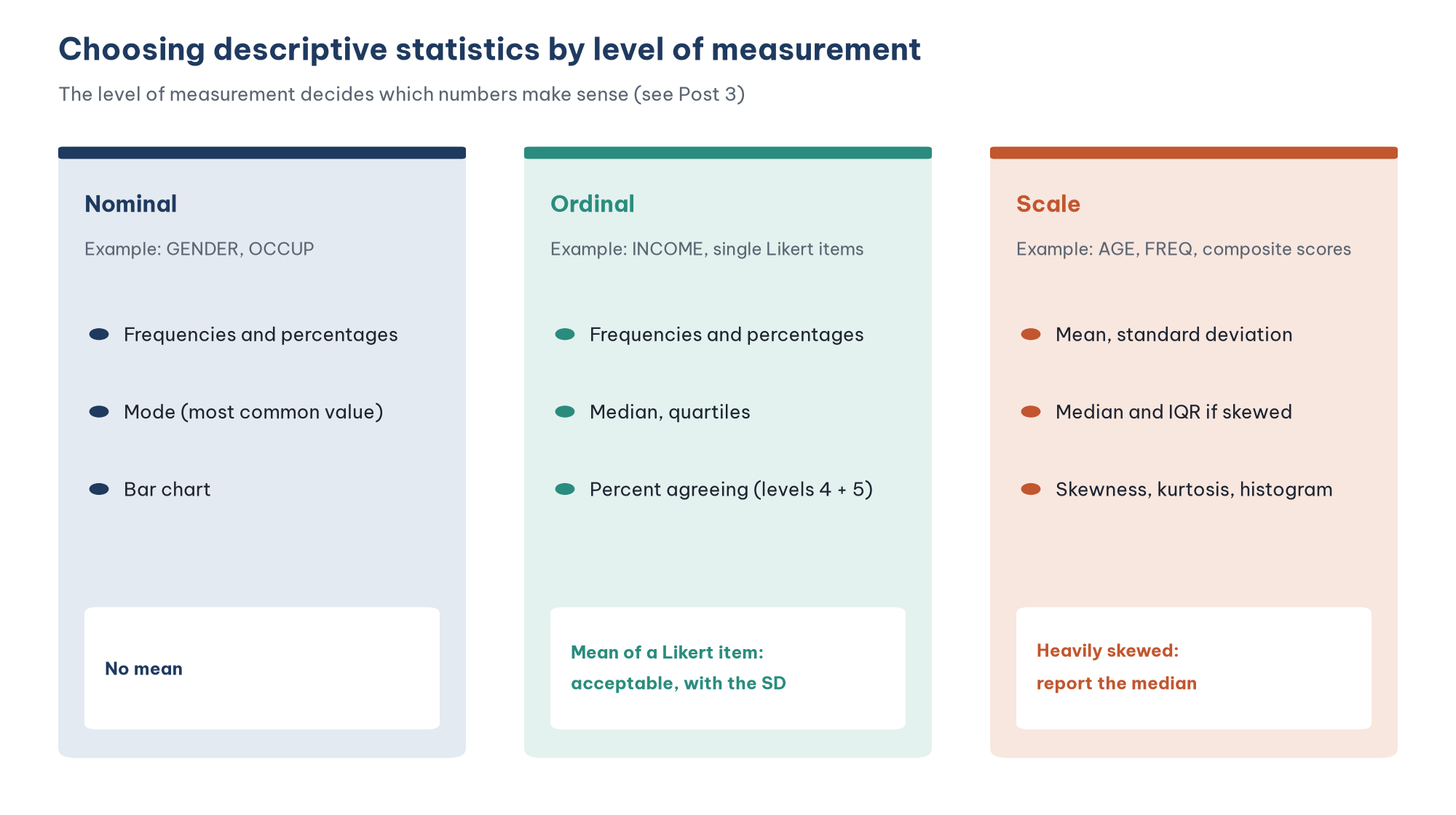
The rule from Post 3, "Levels of Measurement in Research" applies directly here:
Nominal variables (gender, occupation) have only frequencies, percentages and the mode. "Mean gender = 1.55" is a meaningless number.
Ordinal variables (income group) also have the median and quartiles, because the levels are ordered but the distances between them are not equal.
Scale variables (age, number of purchases) can use the mean and standard deviation. If the distribution is heavily skewed, the median and the interquartile range (IQR) describe it more accurately.
Likert items sit in a zone of debate. Jamieson (2004) argues that a Likert item is an ordinal scale, so only the median and frequencies should be reported. On the other hand, Norman (2010) and Carifio and Perla (2007) show that methods based on the mean still give reliable results with Likert data, especially when several items are combined into a scale. Common practice in business research is to report the mean and standard deviation of each item, together with the frequency distribution so the reader can see the shape of the answers. This post follows that practice.
2. Describe the sample with frequency tables
Run FREQUENCIES
In the menus, choose Analyze > Descriptive Statistics > Frequencies and move the demographic variables into the Variable(s) box. Click Charts to request bar charts. The matching syntax is:
FREQUENCIES GENDER OCCUP INCOME /STATISTICS=NONE /BARCHART./STATISTICS=NONE drops the statistics table (mean, standard deviation), which means nothing for a nominal variable.
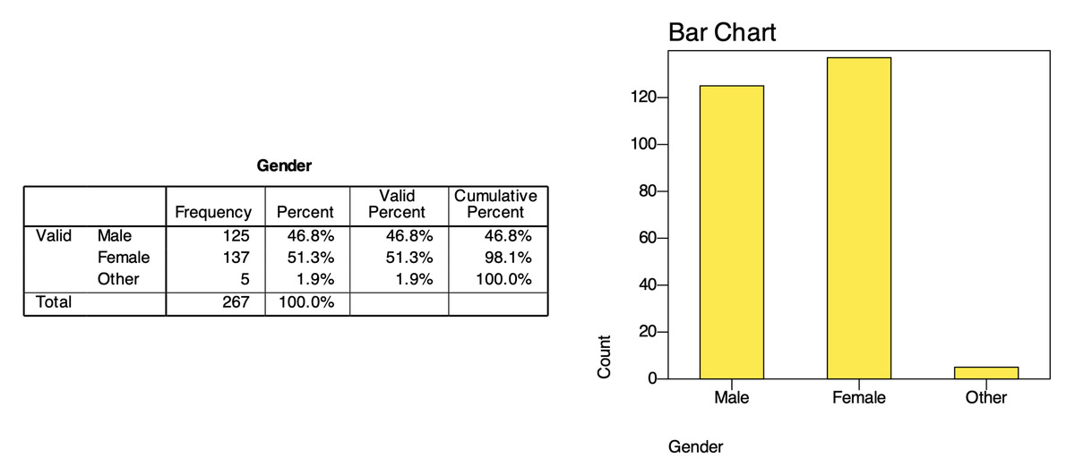
Read the frequency table
A frequency table has four columns of numbers (Table 1).
When a variable has no missing values, Percent and Valid Percent are equal. When there are missing values, report Valid Percent, because it is the share among the people who actually answered the question. The Cumulative Percent column only makes sense for an ordered variable such as income: "61.0% of respondents earn less than $2,000 a month".
Present a sample profile table
In a thesis, the frequency tables are combined into one sample profile table (Table 2).
The commentary should do two things. First, point out what stands out: the sample is fairly balanced by gender, and office workers are the largest group (41.9%). Second, assess representativeness if you have population figures to compare with, such as the customer profile of Marketplace X. Also note groups that are too small: only 5 respondents chose "Other" for gender, so this group cannot be compared with men and women in later analyses.
3. Describe scale variables: age and number of purchases
Run statistics for scale variables
For a scale variable, FREQUENCIES gives more statistics than DESCRIPTIVES, including the median and percentiles. The option /FORMAT=NOTABLE drops the long frequency table (AGE has 38 different values):
FREQUENCIES AGE FREQ /FORMAT=NOTABLE
  /STATISTICS=MEAN MEDIAN STDDEV MINIMUM MAXIMUM SKEWNESS SESKEW KURTOSIS SEKURT
  /PERCENTILES=25 75 /HISTOGRAM=NORMAL.
In the menus, these statistics are under the Statistics button of the Frequencies dialog.
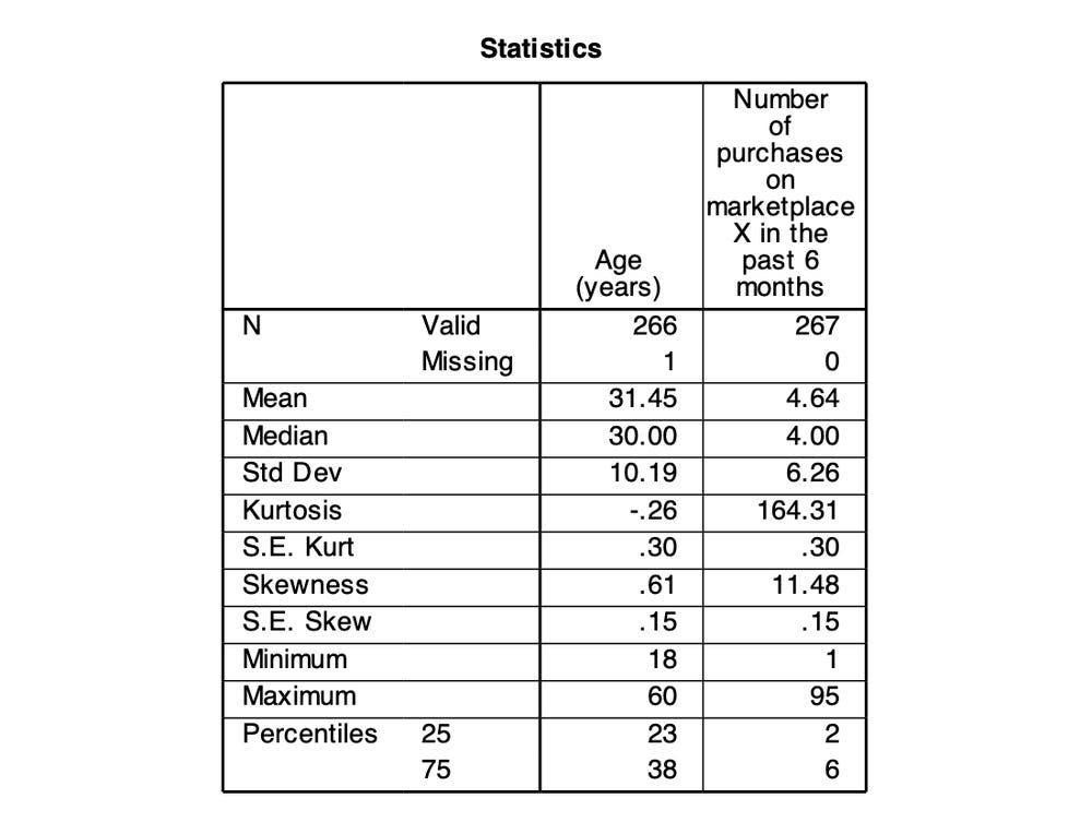
Read the results: mean or median?
Age has a mean of 31.45 and a median of 30. The two numbers are close, which suggests a fairly balanced distribution. A standard deviation of 10.19 years means that roughly two thirds of the respondents are between 21 and 42 years old (the mean plus or minus one standard deviation). Half of the respondents are between 23 and 38 (the first and third quartiles).
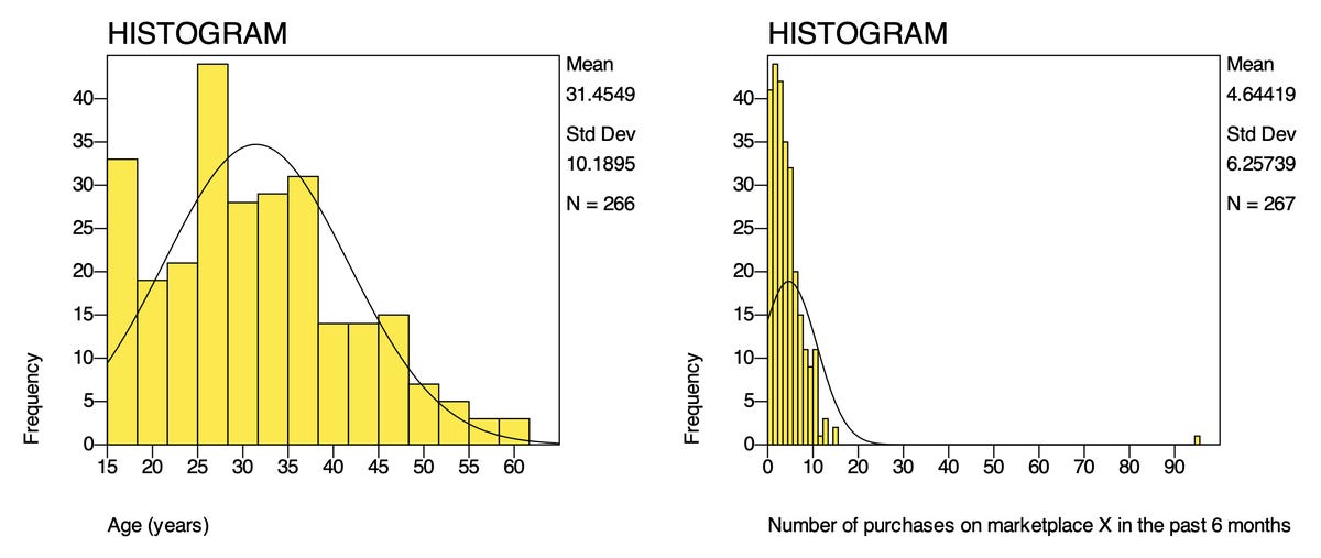
Number of purchases tells a different story. The mean is 4.64 purchases, but the standard deviation is 6.26, larger than the mean itself. This is a sign that the distribution is pulled by an extreme value: response 99, with 95 purchases, which Post 8 decided to keep. Compare the statistics with and without this response (Table 3).
A single response more than doubles the standard deviation, but the median does not change. So for FREQ, report the median and the interquartile range: "The number of purchases on Marketplace X in the past 6 months had a median of 4 (IQR = 2–6)." The two histograms show the difference in shape clearly:
A small note on percentiles: in PSPP 2.1.2 the percentile rows show no decimals (23 and 38 for AGE), while the mean and median have two. In PSPP 2.0, with AGE given two decimals (FORMATS AGE (F5.2).), the first quartile of age shows as 23.25, because PSPP interpolates between neighbouring values. Different programs use slightly different definitions of percentiles and can give slightly different quartiles; that is not an error.
4. Skewness and kurtosis: judging the shape of a distribution
Skewness measures how lopsided a distribution is. A value of 0 means symmetric, a positive value means skewed to the right (a long tail towards large values) and a negative value means skewed to the left. Kurtosis measures how "heavy" the two tails are compared with a normal distribution. PSPP and SPSS report excess kurtosis, so a normal distribution has a kurtosis of 0.
There are two ways to use these two statistics:
Significance test: divide the skewness by its standard error (S.E. Skew) to get a z score. For sample sizes from 50 to 300, Kim (2013) suggests treating a distribution as non-normal when the absolute z is greater than 3.29. This approach is very sensitive to sample size: with a large sample the standard error is small (0.15 with 267 responses), so even a tiny skew becomes statistically significant. For samples above 300, Kim (2013) recommends using the absolute values directly instead of z scores.
Compare with absolute cut-offs: what matters is how much a distribution is skewed, not whether it is skewed at all. West et al. (1995) and Curran et al. (1996) show that estimation methods in structural equation models start to be noticeably affected when the absolute skewness is greater than 2 or the absolute kurtosis is greater than 7. Hair et al. (2022) use a stricter cut-off of ±1 to flag a distribution as clearly skewed.
Table 4 applies the cut-offs to the sample data.
The Likert items are all skewed to the left because most respondents chose "Agree" and "Strongly agree". This is very common in surveys of current customers, people who have already chosen to keep using the service. If you computed z scores (for example CONF1: −0.85 / 0.15 = about −5.7), almost every item would be called "non-normal", yet the amount of skew stays within ±2 and ±7. With the strict ±1 cut-off of Hair et al. (2022), only PV3 has a kurtosis (1.07) slightly above the limit. Normality is discussed further in the FAQ at the end of this post.
5. Describe the Likert items
Table of means and standard deviations
DESCRIPTIVES CONF1 TO SAT2 SAT3 TO RI4
  /STATISTICS=MEAN STDDEV MIN MAX SKEWNESS KURTOSIS.
The variable list skips the attention-check item AC1, which sits between SAT2 and SAT3 in the file and is not a measurement item. Because the items have variable labels, PSPP lists each row by its statement; the rows are, in order, CONF1 to CONF4, PV1 to PV4, SAT1 to SAT4, TRU1 to TRU4 and RI1 to RI4. The table is long, so it runs over two pages of the output and is shown here in three parts.
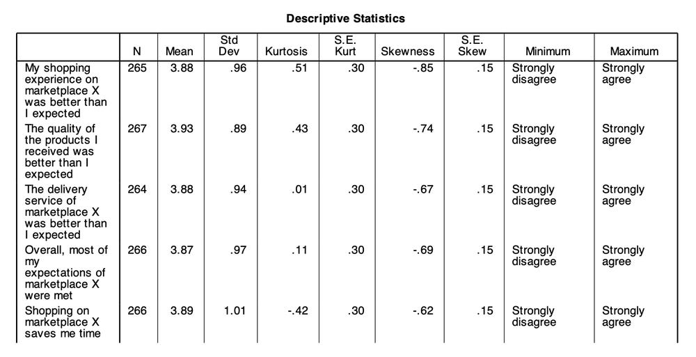
Figure 5a. CONF1 to CONF4 and PV1. In PSPP 2.1.2 the Minimum and Maximum columns show the value labels "Strongly disagree" and "Strongly agree" (codes 1 and 5).
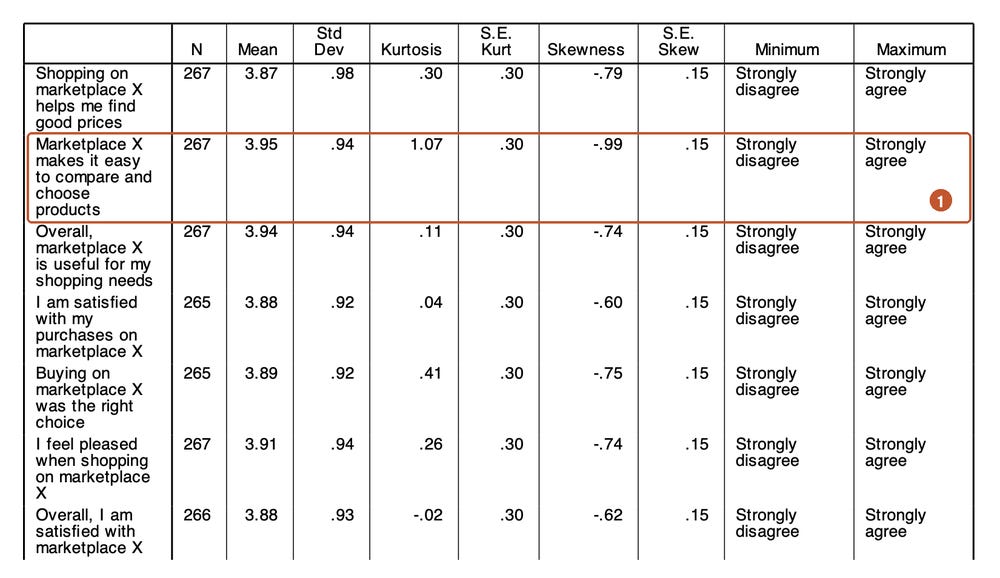
Figure 5b. PV2 to PV4 and SAT1 to SAT4. PV3 has the largest kurtosis (1.07) and the strongest left skew (−0.99) (1).
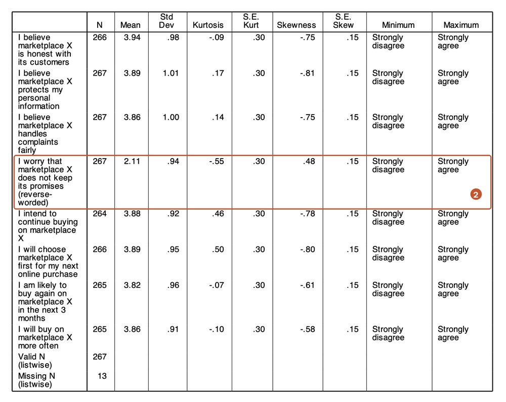
Figure 5c. TRU1 to TRU4 and RI1 to RI4. TRU4 has a mean of only 2.11 because it is a reverse-worded item that has not been recoded yet (2).
Three things to read in this table:
The item means are very close, from 3.82 (RI3) to 3.95 (PV3), leaving TRU4 aside. Overall, respondents agreed with the positive statements about Marketplace X.
Standard deviations range from 0.89 to 1.01. Answers are spread about one level around the mean. If an item had a very small standard deviation (below 0.5), almost everyone would have answered the same way and the item could hardly tell respondents apart.
TRU4 is completely different from the other items, with a mean of 2.11 and a positive skew. This is not a sign that customers lack trust: TRU4 is worded the other way round ("I worry that marketplace X does not keep its promises"). It must be recoded before it is combined into the Trust scale; Post 10, "Recoding Variables and Computing Composite Scores" shows how.
The last two rows of Figure 5c are explained in the FAQ below.
Frequency table of each item
A mean of 3.88 for SAT1 does not tell you how many people are actually satisfied. The frequency table answers that question:
FREQUENCIES SAT1 SAT2 SAT3 SAT4 /STATISTICS=MEDIAN MODE.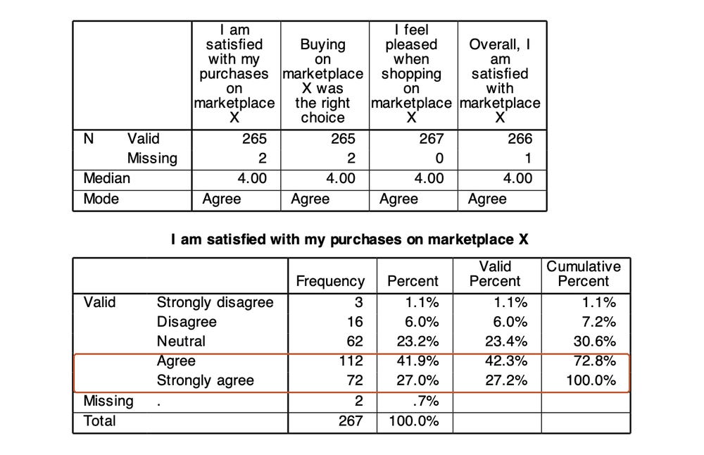
Taking the two highest levels together, 69.4% of respondents are satisfied with their purchases on Marketplace X, 23.4% are neutral and 7.2% are dissatisfied. This way of reporting the share who agree (often called top-2-box) is easy to understand for non-specialist readers and easy to compare between surveys. The median of all four SAT items is 4 and the mode is "Agree" (code 4).
Chart of the answer distribution
With many Likert items, a diverging stacked bar chart gives a quicker overview than a table of numbers. The disagree levels sit to the left of the zero line, the agree levels to the right and the neutral level is split in half across the line:
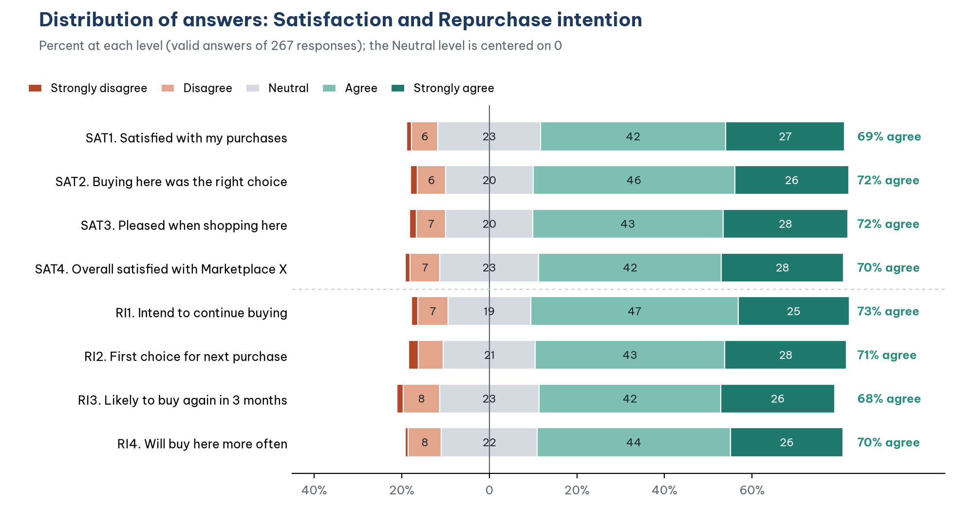
The chart shows that the two scales have almost the same answer pattern. Item RI3, "I am likely to buy again on marketplace X in the next 3 months", has the lowest share agreeing (67.5%) and the highest share disagreeing (9.8%). It asks about a specific behaviour in a specific time frame, so respondents are more careful about committing.
Should you convert means into "high, medium, low"?
Many theses split the 1–5 scale into five equal intervals, each (5 − 1) / 5 = 0.8 wide: 1.00 to 1.80 is "very low", ..., 4.21 to 5.00 is "very high". With this rule, a mean of 3.88 falls into "high". The conversion is convenient but has two weaknesses. First, the boundaries are a convention with no statistical basis: 3.40 is "medium" while 3.41 is "high". Second, it hides the distribution: two items with the same mean of 3.5 can differ completely, one with most answers at 3 and 4, the other split between 1 and 5. If you use it, state clearly that it is a convention and always add the share who agree or a distribution chart.
6. Describe by group
The MEANS command (menu Analyze > Compare Means > Means) computes the mean of a scale variable for each group:
FORMATS AGE FREQ RI1 (F5.2).
MEANS TABLES=AGE FREQ RI1 BY GENDER /CELLS=MEAN COUNT STDDEV.
The FORMATS command in front is needed. The MEANS table shows numbers in the display format of each variable. AGE and FREQ are defined as F3.0 and RI1 as F2.0 (whole numbers), so without FORMATS PSPP prints the mean age as "31" and the standard deviation of RI1 as "1", and information is lost. Figure 8 is exactly that table: the syntax file descriptive_statistics.sps runs MEANS without FORMATS, so you can see the problem for yourself.
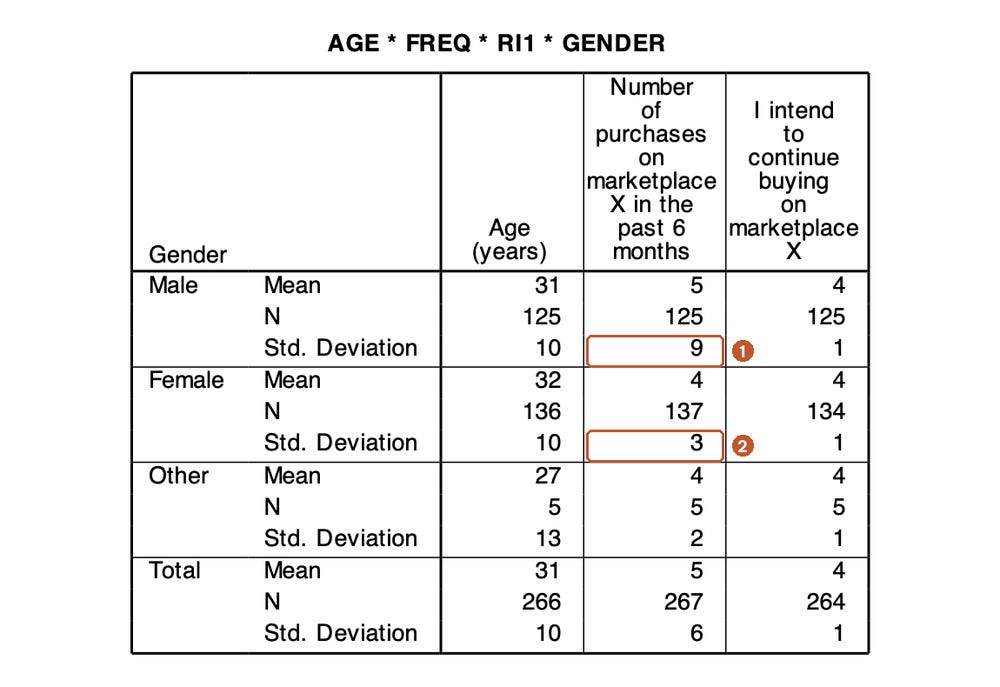
Even rounded, the table shows that the standard deviation of the number of purchases is far larger for men than for women. With two decimals (as PSPP 2.0 prints it with FORMATS in place, and as a check computed from the same data file confirms), it is 8.55 for men against 3.11 for women, almost three times as large. The reason is again response 99: this respondent is a man. Without response 99, the standard deviation for men drops to 2.69. This is an example of why you need to go back to the data-cleaning results when you read descriptive statistics.
Descriptive statistics by group only describe differences in the sample. To conclude that men and women differ in repurchase intention in the population, you need an independent-samples t-test or ANOVA, covered in Post 17, "T-Tests in PSPP (SPSS)" and Post 18, "One-Way ANOVA in PSPP (SPSS)".
The syntax file ends with CROSSTABS /TABLES=OCCUP BY INCOME /CELLS=COUNT ROW., a cross-tabulation of occupation by income with row percentages. It is a quick way to see, for example, that 8.4% of students and 10.7% of office workers earn $3,000 or more a month (the full table is on the last page of raw/pspp-output-post09.pdf).
7. Present descriptive statistics in a report
Some conventions from APA 7 (American Psychological Association, 2020):
The mean is written M, the standard deviation SD and the sample size N (whole sample) or n (subgroup), in italics.
Round means and standard deviations to two decimal places and percentages to one.
Do not repeat in the text every number already in a table. The text only points out what stands out.
Use a decimal point (3.88) and keep the number of decimals consistent throughout.
A table describing the measurement items usually looks like Table 5.
Sample paragraph: "The Satisfaction items had means from 3.88 to 3.91 (SD from 0.92 to 0.94), showing that respondents were generally satisfied with Marketplace X: 69% to 72% of respondents chose Agree or Strongly agree. The skewness of the 20 measurement items ranged from −0.99 to 0.48 and the kurtosis from −0.55 to 1.07, all below the cut-offs of |2| and |7| of West et al. (1995)."
Five common mistakes
Computing a mean for a nominal variable, such as "mean gender 1.55" or "mean occupation 2.06".
Reporting only the mean for a heavily skewed variable such as FREQ, without the median, so the reader thinks a typical respondent bought almost 5 times.
Using Percent instead of Valid Percent when there are missing values, so the group percentages do not add up to 100%.
Reading a reverse-worded item as a normal item, for example concluding "customers have low trust" from the mean of 2.11 for TRU4.
Forgetting FORMATS before MEANS, so the means are rounded to whole numbers in the output table (Figure 8).
Frequently asked questions
Should I run descriptive statistics for every item, or only for the composite variables?
Do both. Describing each item helps you find problem items, such as a reverse-worded item that has not been recoded or an item with a very small standard deviation. The composite variables (the mean of the items in a scale) are described after the reliability check in Post 11, "Cronbach's Alpha in PSPP (SPSS)" and after they are computed in Post 10.
What is the difference between DESCRIPTIVES and FREQUENCIES?
DESCRIPTIVES is quick and compact when you need the mean and standard deviation of many variables in one table, and it has an option to save z scores, as used in Post 8. FREQUENCIES adds the frequency table, median, mode, percentiles and charts. For nominal and ordinal variables, always use FREQUENCIES.
Why does PSPP show Valid N (listwise) = 267 when only 254 responses are complete?
The PSPP DESCRIPTIVES table puts the total number of responses in the Valid N (listwise) row and the number of responses missing at least one of the variables in the Missing N (listwise) row, here 13 (Figure 5c). The number of complete responses is 267 − 13 = 254. SPSS prints 254 directly in the Valid N (listwise) row.
Do I need a normality test (Shapiro-Wilk, Kolmogorov-Smirnov) for each item?
No, and the result would not mean much. A 5-point Likert item has only 5 discrete values, so it can never be normally distributed, and with a sample of a few hundred the test almost always gives p < .001 for every item. What you need to know is how much the distribution is skewed, so report the skewness and kurtosis of each item as in section 5 and compare them with |2| and |7| (West et al., 1995). Whether you need to look at the distribution at all depends on the analysis (Table 6).
For the sample data, the table in Figures 5a to 5c shows that the 20 items have skewness from −0.99 to 0.48 and kurtosis from −0.55 to 1.07, within the cut-offs. That is enough evidence for the data description. Mardia's coefficient is checked in Post 22, "Confirmatory Factor Analysis (CFA) in JASP".
References
American Psychological Association. (2020). Publication manual of the American Psychological Association (7th ed.). https://doi.org/10.1037/0000165-000
Bentler, P. M. (2005). EQS 6 structural equations program manual. Multivariate Software.
Carifio, J., & Perla, R. J. (2007). Ten common misunderstandings, misconceptions, persistent myths and urban legends about Likert scales and Likert response formats and their antidotes. Journal of Social Sciences, 3(3), 106–116. https://doi.org/10.3844/jssp.2007.106.116
Curran, P. J., West, S. G., & Finch, J. F. (1996). The robustness of test statistics to nonnormality and specification error in confirmatory factor analysis. Psychological Methods, 1(1), 16–29. https://doi.org/10.1037/1082-989X.1.1.16
Free Software Foundation. (2026). GNU PSPP (Version 2.1.2) [Computer software]. https://www.gnu.org/software/pspp/
Hair, J. F., Hult, G. T. M., Ringle, C. M., & Sarstedt, M. (2022). A primer on partial least squares structural equation modeling (PLS-SEM) (3rd ed.). SAGE Publications.
Jamieson, S. (2004). Likert scales: How to (ab)use them. Medical Education, 38(12), 1217–1218. https://doi.org/10.1111/j.1365-2929.2004.02012.x
Kim, H.-Y. (2013). Statistical notes for clinical researchers: Assessing normal distribution (2) using skewness and kurtosis. Restorative Dentistry & Endodontics, 38(1), 52–54. https://doi.org/10.5395/rde.2013.38.1.52
Norman, G. (2010). Likert scales, levels of measurement and the "laws" of statistics. Advances in Health Sciences Education, 15(5), 625–632. https://doi.org/10.1007/s10459-010-9222-y
West, S. G., Finch, J. F., & Curran, P. J. (1995). Structural equation models with nonnormal variables: Problems and remedies. In R. H. Hoyle (Ed.), Structural equation modeling: Concepts, issues, and applications (pp. 56–75). SAGE Publications.
Discussion about this post