T-Tests in PSPP (SPSS): Independent, Paired and One-Sample Tests
Run the independent, paired and one-sample t-tests in PSPP or SPSS, prefer Welch, compute Cohen’s d and read a non-significant result


Key takeaways
Where the two means come from decides the test: one variable against a given number, two independent groups or two measurements on the same people.
Read the Welch row by default: for FREQ, Levene's test gives p = 0.523 even though the standard deviation of one group is almost three times that of the other.
PSPP prints no effect size, so the syntax computes Cohen's d with AGGREGATE (d = −0.004 for repurchase intention by gender); sort the cases first or the pooled SD can be wrong.
Mann-Whitney and Wilcoxon tests lead to the same conclusions as the t-tests and serve as robustness checks.
A non-significant result is not proof of no difference: read the confidence interval and use an equivalence test (TOST) with a bound set in advance.
After the regressions of the previous posts, many research questions are actually simpler: do men and women differ in repurchase intention? Do customers rate two perceived-value questions the same way? Does mean satisfaction reach the target of 4 points set by the customer care team of marketplace X? All three questions compare means, and the standard tool to answer them is the t-test (Field, 2024).
This post covers all three types of t-test on the sample data set (marketplace_x_analysis.sav, 267 respondents). Every result comes from the syntax file t_test.sps from the GitHub repository of this post, run in PSPP (Free Software Foundation, 2026), and is checked again with Python (check_python.py). Two of the tests are not significant. The post keeps those results as they are and uses them to show how to read a "no difference" result correctly.
Sample data and scripts. The data files and scripts for this post are in the research-data-analysis repository on GitHub (folder
data/andscripts/). Download the whole repository with Code > Download ZIP.
About the figures. Figures 3 to 6 are real screenshots of PSPP 2.1.2 on macOS (Apple silicon Mac), taken in November 2026 with the data file
marketplace_x_analysis.sav(in thedata/folder of the repository). Figures 2, 7, 8 and 9 are real output oft_test.sps, run in PSPP 2.1.2 and exported from the Output Viewer (File > Export > PDF); tables that run over two pages of the export are joined, and no value is changed. Figure 10 is drawn with Python from the sample data.
1. Choose the right type of t-test
Only one question decides it: where do the two means you want to compare come from?
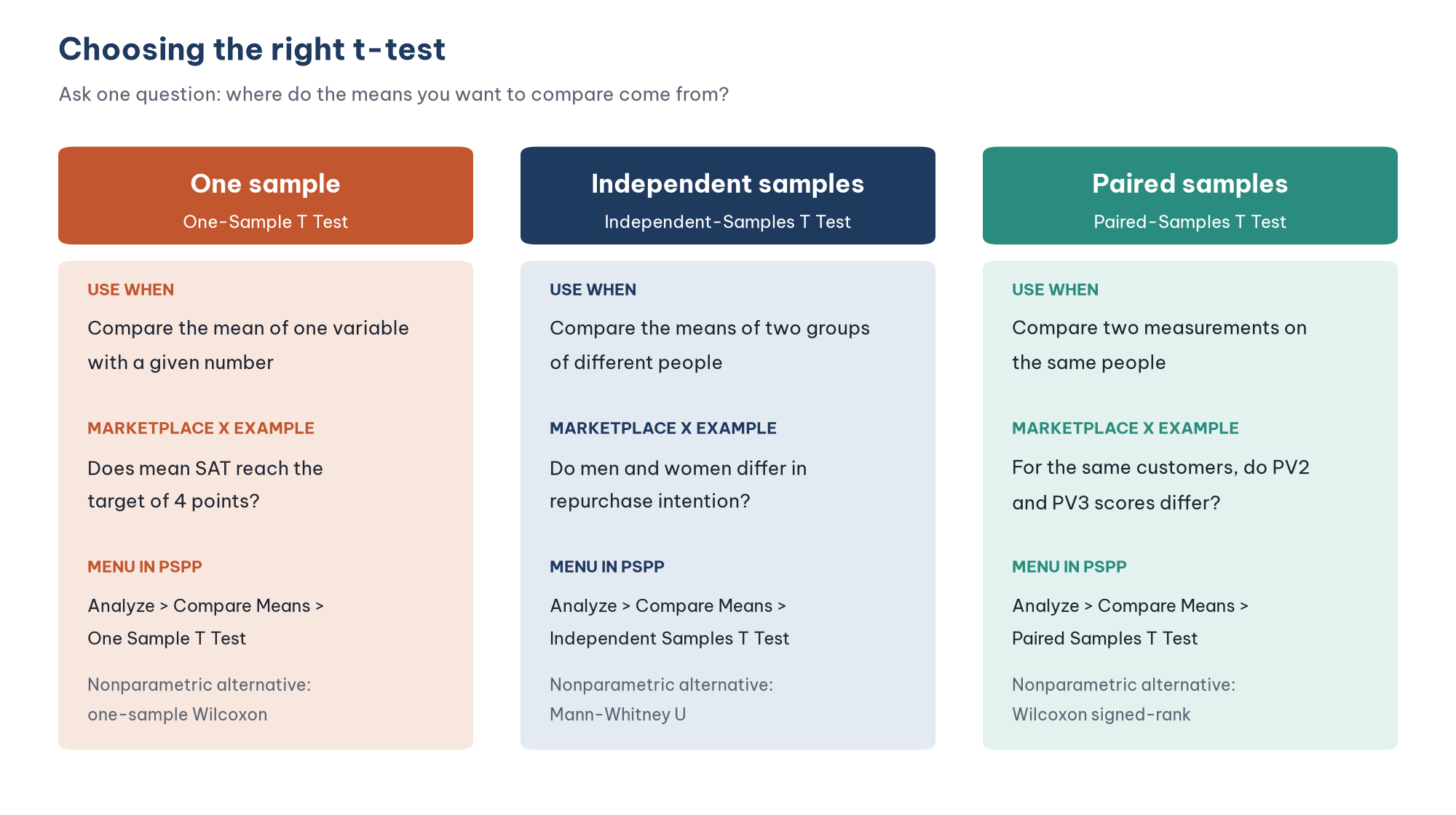
Table 1 summarizes the three types.
A very common mistake is to use the independent-samples test for paired data, for example to compare the scores of the same group of employees before and after a training course. Paired data have a correlation between the two measurements. The independent test ignores that correlation, so the standard error is estimated wrongly. If the same person answers both variables, use the paired-samples test.
If the grouping variable has three or more groups (for example four occupation groups), do not run a t-test for every pair, because the type I error accumulates. Use one-way ANOVA in Post 18, "One-Way ANOVA in PSPP (SPSS) and Post-Hoc Tests" instead.
2. Assumptions of the t-test
Check that the dependent variable is quantitative. The mean score of a Likert scale (such as RI or SAT) is treated as quantitative. A single Likert question (such as PV2) has only five levels, so with the paired test you should also run a nonparametric test as a cross-check (Section 5).
Check that the observations are independent. Each respondent appears only once in each group. In the independent test, one person cannot belong to both groups.
Check that the distribution is not too skewed. The t-test is quite robust when each group has about 30 cases or more, thanks to the central limit theorem (Lumley et al., 2002). What matters is strong outliers, not the result of the Shapiro-Wilk test (see the FAQ of Post 9, "Descriptive Statistics in PSPP (SPSS)").
Check the variances of the two groups (independent test only). Section 3 explains why this post recommends reading the Welch result by default.
A box plot is the quickest way to check assumptions 3 and 4 at the same time. Menu: Analyze > Descriptive Statistics > Explore, move RI into the Dependent List and GENDER into the Factor List and choose Plots > Boxplots.
EXAMINE VARIABLES=RI BY GENDER /PLOT=BOXPLOT /STATISTICS=NONE.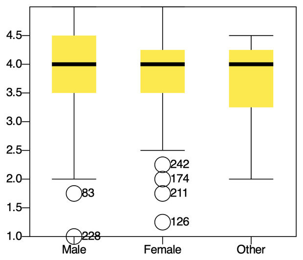
The Male and Female boxes have the same median (4.0) and a similar spread (the box runs from 3.5 to 4.5 for men and from 3.5 to 4.25 for women). There are a few low outliers, labeled 83 and 228 among the men and 242, 174, 211 and 126 among the women. As explained in Post 8, "Data Cleaning in PSPP (SPSS)", these labels are row numbers, not response IDs (rows 83, 228, 242, 174, 211 and 126 are responses 92, 256, 271, 196, 236 and 139); add /ID=ID to the command to label by ID. The outliers are not very far from the rest, and both groups have more than 120 people, so the t-test is still appropriate.
In PSPP 2.1.2 this EXAMINE command also prints a Case Processing Summary (125 men, 135 women with RI, 5 Other; 2 women have no RI score) and a Tests of Normality table with the Shapiro-Wilk test, even with /STATISTICS=NONE. As noted in assumption 3, a significant Shapiro-Wilk result in groups of this size is not a reason to drop the t-test.
3. Independent-samples t-test
Run the test in PSPP
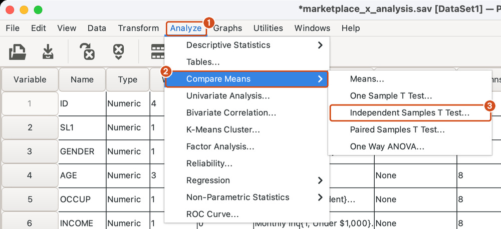
Open Analyze > Compare Means > Independent Samples T Test (Figure 3).
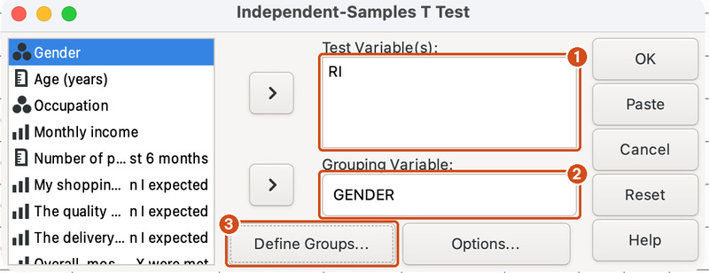
Move RI into the Test Variable(s) box and GENDER into the Grouping Variable box (Figure 4).
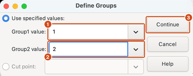
Click Define Groups, keep Use specified values selected and enter the codes of the two groups to compare: Group1 value = 1 (Male), Group2 value = 2 (Female), then click Continue (Figure 5).
Click Paste to get the syntax (Figure 6), or OK to run the test straight away.

The syntax file t_test.sps runs the test for three variables at once, to give more examples:
T-TEST /VARIABLES=RI SAT FREQ
  /GROUPS=GENDER(1,2)
  /MISSING=ANALYSIS
  /CRITERIA=CI(0.95).
/MISSING=ANALYSIS drops missing values variable by variable, so each variable uses as many respondents as possible. The five people who chose "Other" are left out because they are coded neither 1 nor 2. This group is too small to compare on its own; if needed, report its descriptive statistics separately rather than merging it into another group at will.
Read the results
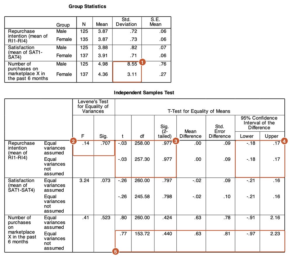
Read the tables in five steps:
Read the Group Statistics table. RI is 3.87 for men (SD = 0.72; n = 125) and 3.87 for women (SD = 0.73; n = 135). The two means almost coincide.
Read Levene's test (box 2). F = 0.14; p = 0.707: no evidence that the variances of the two groups differ.
Read the t row (box 3). t = −0.03; p = 0.977. The Equal variances assumed and Equal variances not assumed rows give almost the same result, because the variances and group sizes are similar (258 versus 257.30 degrees of freedom).
Read the confidence interval (box 4). The difference, men minus women, lies between −0.18 and 0.17 points. The interval contains 0. PSPP shows the Mean Difference as .00 because it rounds to two decimals; the exact value is −0.003 (3.865 − 3.868, see the Cohen's d output below).
Conclude. There is no evidence that repurchase intention differs between men and women.
Levene or Welch: which row should you read?
The traditional teaching is: if Levene's test has p > 0.05, read the Equal variances assumed row (Student's test); otherwise read the not assumed row (Welch's test). This two-step procedure has two problems (Delacre et al., 2017):
Levene's test has low power in small samples, so it often "fails to detect" unequal variances even when they really differ.
Welch's test loses almost no accuracy when the variances are equal, but it avoids large errors when the variances differ and the group sizes are unequal.
The variable FREQ (number of purchases in the past 6 months) shows the first problem clearly. The standard deviation for men is 8.55, almost three times that for women (3.11) (box 1). Yet Levene's test gives p = 0.523. The cause is a single respondent (response ID 99, a man who reported 95 purchases, kept after the check in Post 8). Levene's test compares the absolute deviations from the mean between the two groups. This extreme value raises the mean deviation of the male group, but it also greatly raises the variability of those deviations within the male group, so Levene's F stays small. With response ID 99 removed, the standard deviation of the male group is only 2.69.
For FREQ, the Welch row (box 5) gives t(153.72) = 0.77; p = 0.440, and the Student row gives p = 0.424. The conclusion does not change in this example, but the Welch degrees of freedom drop sharply (153.72 versus 260) because the test recognizes that the male group is less precise.
Recommendation of this post: read the Equal variances not assumed (Welch) row by default, and report its fractional degrees of freedom. Simply state in the method section that you used Welch's test.
Compute the Cohen's d effect size
The p value only tells you whether there is enough evidence of a difference, not how large the difference is. Cohen's d measures the mean difference in units of the pooled standard deviation (Cohen, 1988; Lakens, 2013):
d = (mean of group 1 − mean of group 2) / pooled SD
pooled SD = square root of [(n1 − 1) × SD1² + (n2 − 1) × SD2²] / (n1 + n2 − 2)
where n1 and n2 are the sample sizes and SD1 and SD2 the standard deviations of group 1 and group 2.
Cohen's (1988) rough benchmarks: 0.2 is small, 0.5 is medium and 0.8 is large. Comparing with studies in the same field is better than applying these benchmarks mechanically.
PSPP does not print Cohen's d (the T-TEST output of PSPP 2.1.2 has no effect size). The file t_test.sps computes d with AGGREGATE:
DATASET COPY CALC_D.
DATASET ACTIVATE CALC_D.
SELECT IF ANY(GENDER, 1, 2) AND NOT MISSING(RI).
* AGGREGATE by group needs the data sorted by the grouping variable first.
SORT CASES BY GENDER.
AGGREGATE /OUTFILE=* MODE=ADDVARIABLES /BREAK=GENDER /M_GROUP=MEAN(RI).
IF (GENDER = 1) RI_MALE = RI.
IF (GENDER = 2) RI_FEMALE = RI.
COMPUTE SQ_DEV = (RI - M_GROUP) ** 2.
AGGREGATE /OUTFILE=* MODE=ADDVARIABLES /M_MALE=MEAN(RI_MALE) /M_FEMALE=MEAN(RI_FEMALE)
  /SS_WITHIN=SUM(SQ_DEV) /N_TOTAL=N(RI).
COMPUTE SD_POOLED = SQRT(SS_WITHIN / (N_TOTAL - 2)).
COMPUTE COHEN_D = (M_MALE - M_FEMALE) / SD_POOLED.
Result (the Data List table in the output): N = 260, mean for men 3.865, mean for women 3.868, pooled SD = 0.726, d = −0.004. The difference between men and women is practically zero.
Note the SORT CASES line. When an earlier version of this syntax was tested in PSPP 2.0 without sorting first, AGGREGATE with /BREAK gave a wrong pooled SD (0.551 instead of 0.726) without any error message. Always check against another method; here the value is checked again with Python.
In SPSS from version 27, the t-test dialogs have an Estimate effect sizes box that prints Cohen's d and Hedges' g.
4. Paired-samples t-test
The situation
The Perceived value (PV) scale has two items: PV2 "Shopping on marketplace X helps me find good prices" and PV3 "Marketplace X makes it easy to compare and choose products". The marketing team wants to know whether customers rate these two benefits the same way. The same person answers both items, so the data are paired.
Run the test
Open Analyze > Compare Means > Paired Samples T Test.
Choose PV2 as Variable 1 and PV3 as Variable 2 of the first pair.
Click OK or Paste.
T-TEST /PAIRS=PV2 WITH PV3 (PAIRED) /CRITERIA=CI(0.95).Read the results
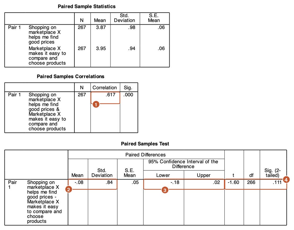
Read the Paired Sample Statistics table. PV2 = 3.87; PV3 = 3.95; N = 267.
Read the correlation table (box 1). r = 0.617: people who rate one item high usually rate the other high too. This positive correlation is why the paired test has a smaller standard error than the independent test.
Read the difference (box 2). PV2 minus PV3 is −0.08 points on average (SD = 0.84).
Read the confidence interval (box 3): from −0.18 to 0.02, which contains 0.
Read t and Sig. (box 4): t(266) = −1.60; p = 0.111.
Conclude. There is not enough evidence to say that customers rate these two benefits differently.
The effect size for paired data is d*z = mean difference / *SD of the differences = −0.08 / 0.84 = −0.10 (Lakens, 2013). PSPP does not print it, but you can compute it by hand from the table, or with COMPUTE DIFF_PV = PV2 - PV3. followed by DESCRIPTIVES as in the syntax file (mean −0.08, SD 0.84, N = 267).
5. Nonparametric alternatives
When the sample is small and the distribution very skewed, or when the variable has only a few levels like a single Likert question, run a nonparametric test as a cross-check (Table 2).
NPAR TESTS /M-W=RI BY GENDER(1 2).
NPAR TESTS /WILCOXON=PV2 WITH PV3 (PAIRED).
Both nonparametric tests lead to the same conclusion as the t-tests. When the two approaches agree, report the t-test as the main result and mention the nonparametric test as a robustness check. When they disagree, look for the cause (usually outliers) before deciding which result to report. Never choose a test just because it gives p < 0.05.
The Wilcoxon test ignores tied pairs. Here 134 of the 267 people (50%) gave PV2 and PV3 the same score, so the test is based on the remaining 133 people only. This is typical of five-point Likert questions.
6. One-sample t-test
Choose a meaningful test value
The one-sample test compares a mean with a given number (the Test Value). That number must come from the research question, not be picked at will. Two common choices:
The scale midpoint (3). It answers the question "do customers lean toward agreeing or disagreeing?". In the sample data, SAT and RI are both clearly above 3 (t(265) = 19.21 and t(264) = 19.24; both p < .001; d = 1.18). This result is almost obvious when the mean is already 3.9, so it carries little information.
A management target (4). Suppose the customer care team of marketplace X has set a target of a mean satisfaction score of 4 ("Agree"). This question is more useful for decision-making.
Run the test
Open Analyze > Compare Means > One Sample T Test.
Move SAT and RI into the Test Variable(s) box.
Enter 4 in the Test Value box.
Click OK or Paste.
T-TEST /TESTVAL=4 /VARIABLES=SAT RI /CRITERIA=CI(0.95).Read the results
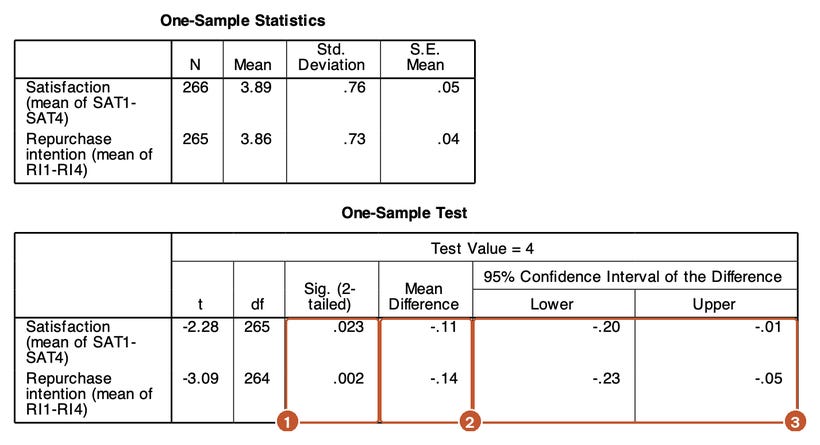
Read the One-Sample Statistics table. SAT = 3.89 (SD = 0.76; N = 266); RI = 3.86 (SD = 0.73; N = 265).
Read Sig. (box 1). SAT: t(265) = −2.28; p = 0.023. RI: t(264) = −3.09; p = 0.002.
Read the difference (box 2). SAT is 0.11 points below the target; RI is 0.14 points below.
Read the confidence interval (box 3). SAT: from −0.20 to −0.01; RI: from −0.23 to −0.05. Both intervals lie entirely below 0.
Conclude. Mean satisfaction and mean repurchase intention do not yet reach the target of 4 points.
Interpretation for managers
The result is statistically significant, but the gap is small: d = −0.14 for SAT and −0.19 for RI, below Cohen's "small" benchmark. The confidence interval for SAT shows that the real shortfall could be as little as 0.01 points or as large as 0.20 points. A suitable way to put it to managers is: "The mean satisfaction score is 3.89, about 0.1 points below the target. The gap is not large, but it is clear enough to say that the target has not been reached." Do not write "customers are dissatisfied", because the mean is still well above the scale midpoint.
7. Read a non-significant result correctly
Two of the four main tests in this post are not significant. Figure 10 puts all four results on the same axis for comparison.
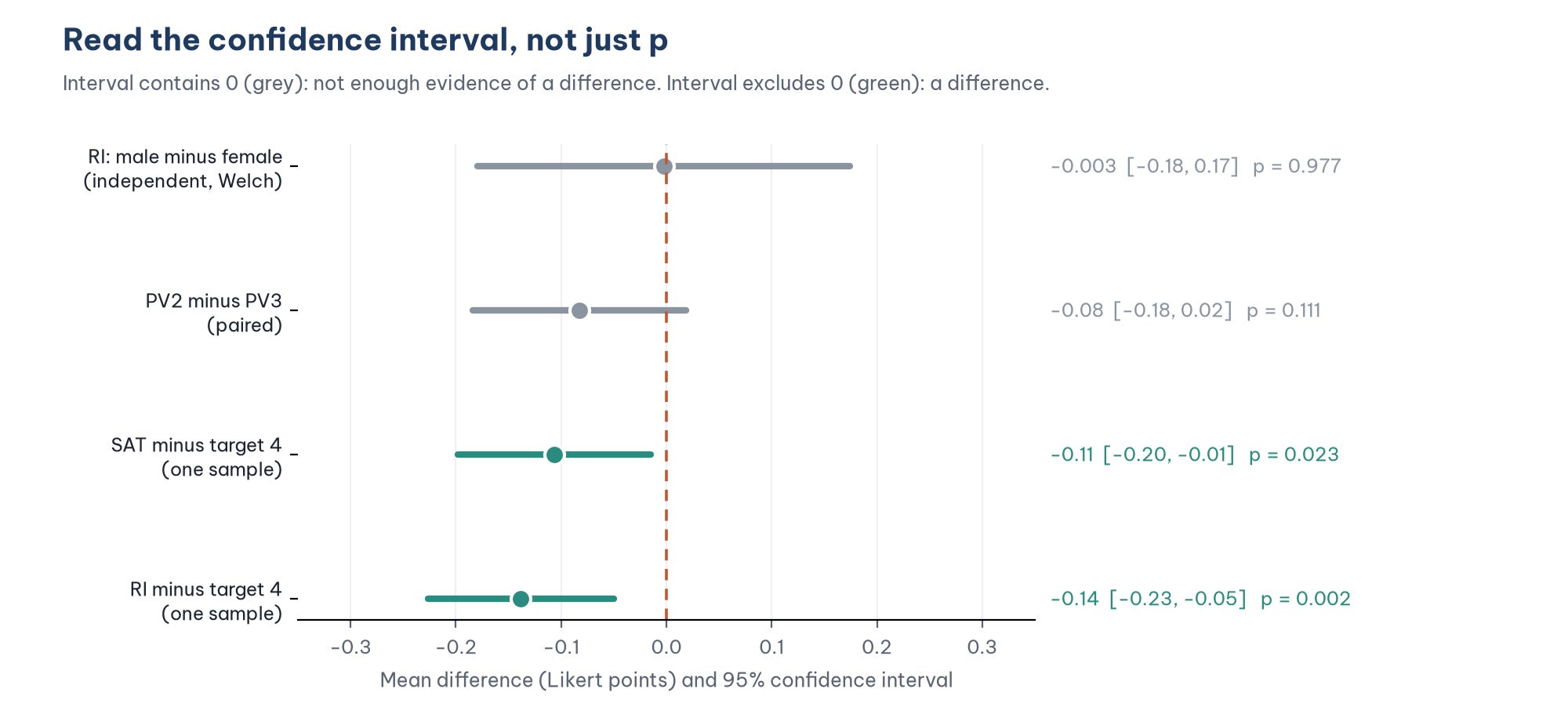
Do not write "men and women have the same repurchase intention". p = 0.977 only tells you that the data do not give enough evidence of a difference. Not being statistically significant does not mean that you have proven there is no difference.
Read the confidence interval to see how tight the "no difference" result is. The confidence interval of RI by gender is [−0.18, 0.17]: the real difference, if any, is almost certainly smaller than 0.2 points on a 5-point scale. The confidence interval of PV2 minus PV3 is [−0.18, 0.02]: it is still possible that PV3 is rated about 0.1 to 0.2 points higher than PV2, and this sample is not large enough to detect it. Both results are "not significant", but their degree of certainty differs.
Use an equivalence test if you want to claim "no difference". If the researcher decides in advance that a difference smaller than 0.2 points is of no practical importance, a two one-sided tests procedure (TOST) can be run (Lakens, 2017). An equivalent check is whether the 90% confidence interval lies entirely within [−0.2, 0.2]. For RI by gender, the 90% confidence interval is [−0.15, 0.15], entirely inside this range (the two one-sided tests give p = 0.015 and 0.013; computed in check_python.py). Only then can you write: "Men and women have equivalent repurchase intention within ±0.2 points." The ±0.2 bound must be chosen and justified before looking at the data.
Do not try more variables until something is significant. Running t-tests by gender for dozens of variables and reporting only those with p < 0.05 is "fishing" for results. If you really need to test many variables, report them all and adjust the significance level (for example Bonferroni: divide 0.05 by the number of tests).
8. Reporting the results in APA 7 style
Independent samples:
An independent-samples t-test (Welch correction) showed no difference in repurchase intention between men (M = 3.87, SD = 0.72, n = 125) and women (M = 3.87, SD = 0.73, n = 135), t(257.30) = −0.03, p = .977, mean difference = −0.003, 95% CI [−0.18, 0.17], d = −0.004. A Mann-Whitney test led to the same conclusion (U = 8401.5, p = .952).
Paired samples:
Ratings of the good-price benefit (PV2: M = 3.87, SD = 0.98) and the easy-comparison benefit (PV3: M = 3.95, SD = 0.94) did not differ significantly, t(266) = −1.60, p = .111, mean difference = −0.08, 95% CI [−0.18, 0.02], *d*z = −0.10.
One sample:
Mean satisfaction (M = 3.89, SD = 0.76) was significantly below the target of 4 points, t(265) = −2.28, p = .023, mean difference = −0.11, 95% CI [−0.20, −0.01], d = −0.14. Repurchase intention (M = 3.86, SD = 0.73) was also below the target, t(264) = −3.09, p = .002, difference = −0.14, 95% CI [−0.23, −0.05], d = −0.19.
Under APA 7, p is reported with two or three decimal places and without a leading zero (p = .023), as in the examples above. Follow the rules of the journal or institution you submit to.
Five common mistakes
Using the independent test for paired data. Before-and-after data, or two questions answered by the same person, need the paired-samples test.
Running several t-tests instead of ANOVA. With three or more groups, use one-way ANOVA (Post 18).
Reading only the Student row because Levene's test has p > 0.05. Levene's test can miss unequal variances, as the FREQ example shows. Read the Welch row by default.
Concluding "no difference" from p > 0.05. Read the confidence interval, and use an equivalence test if you want to claim that two groups are the same.
Reporting only p and leaving out the effect size. With a large sample, even a tiny difference can be statistically significant. Always report the difference, its confidence interval and Cohen's d.
Frequently asked questions
Can I run a t-test when the two groups have very different sizes?
Yes, but use the Welch result. Student's test is most likely to go wrong when the smaller group has the larger variance (Delacre et al., 2017).
Can I use a t-test on a single Likert question?
You can, and in practice with a sample of a few hundred people the result is usually the same as the nonparametric test, as in the PV2 versus PV3 example. Still, run a Mann-Whitney or Wilcoxon test as a cross-check, and prefer to analyze the mean score of the whole scale.
One-tailed or two-tailed t-test?
PSPP and SPSS print the two-tailed Sig. Use a one-tailed test only when the direction of the hypothesis is set in advance and a result in the opposite direction would be meaningless for the research question. In that case the one-tailed p equals the two-tailed p divided by 2, provided the difference is in the expected direction. In a thesis, keep the two-tailed test unless there is a clear reason.
Is a t-test the same as a regression with one dummy variable?
Yes. Regressing RI on a gender dummy (Male = 1, Female = 0) gives a coefficient equal to the mean difference and a t equal to the Student row. It is the same linear model, as you saw with dummy variables in Post 16, "Dummy Variables and Moderator Variables in Regression".
References
Cohen, J. (1988). Statistical power analysis for the behavioral sciences (2nd ed.). Lawrence Erlbaum Associates.
Delacre, M., Lakens, D., & Leys, C. (2017). Why psychologists should by default use Welch's t-test instead of Student's t-test. International Review of Social Psychology, 30(1), 92–101. https://doi.org/10.5334/irsp.82
Field, A. (2024). Discovering statistics using IBM SPSS Statistics (6th ed.). SAGE Publications.
Free Software Foundation. (2026). GNU PSPP (Version 2.1.2) [Computer software]. https://www.gnu.org/software/pspp/
Lakens, D. (2013). Calculating and reporting effect sizes to facilitate cumulative science: A practical primer for t-tests and ANOVAs. Frontiers in Psychology, 4, Article 863. https://doi.org/10.3389/fpsyg.2013.00863
Lakens, D. (2017). Equivalence tests: A practical primer for t tests, correlations, and meta-analyses. Social Psychological and Personality Science, 8(4), 355–362. https://doi.org/10.1177/1948550617697177
Lumley, T., Diehr, P., Emerson, S., & Chen, L. (2002). The importance of the normality assumption in large public health data sets. Annual Review of Public Health, 23, 151–169. https://doi.org/10.1146/annurev.publhealth.23.100901.140546
Discussion about this post