


Key takeaways
Simpson's paradox occurs when a trend holds in every group but weakens or reverses once the groups are combined. Both sets of figures are arithmetically correct.
It needs three conditions at once: a lurking variable that affects the outcome, a different group composition between the options, and enough imbalance to tip the weighted average.
The data alone cannot tell you whether to trust the aggregated or the stratified figures. The causal role of the grouping variable (confounder, mediator or collider) decides.
A regression coefficient has no causal meaning until the causal structure behind it is stated.
Prevent it by design (randomization, stratified randomization, SRM checks), detect it in analysis (compare group composition first), and choose the figure that matches the question.
Imagine you run a hospital. The report on your desk compares two treatments for kidney stones: treatment A succeeds 78% of the time, treatment B 83%. The choice looks clear: pick B.
Then a doctor on the board asks to split the figures by stone size. The result silences the room: for small stones, A beats B; for large stones, A also beats B. How can A win in every group and still lose when the groups are combined?
This is Simpson's paradox. It has reversed conclusions in medicine, education, sports, business and even lawsuits. This article answers four questions in turn: what Simpson's paradox is and why it happens; where it shows up in practice; whether to trust the aggregated or the stratified figures when it appears; and how to detect, handle and prevent it systematically. Section 1 defines the paradox and reviews its history. Section 2 dissects the kidney stone example, and Section 3 presents five real-world cases. Section 4 tackles the key question: aggregate or stratify, with a business example read through a causal diagram. The next three sections cover prevention through study design, detection during analysis, and correct handling once the paradox is found. Section 8 summarizes where the paradox tends to appear in each field, and Section 9 answers some common questions.
1. What is Simpson's paradox?
Simpson's paradox occurs when a trend appears consistently within each group of data but weakens, disappears or reverses when the groups are combined (Simpson, 1951; Blyth, 1972).
It is not a logical contradiction. Both the aggregated and the stratified figures are arithmetically correct. What gets fooled is intuition: we assume that if A beats B in every group, A must beat B overall. That intuition fails in one specific situation, when the options being compared have different group compositions. The next section shows exactly how.
1.1. A brief history
The paradox bears Simpson's name, but Simpson was not the first to notice it. The four milestones below show that it was recognized as early as the end of the 19th century.
1899: Pearson and colleagues noted that mixing heterogeneous groups can produce spurious correlations (Pearson et al., 1899).
1903: Yule analysed similar cases in his work on the association of attributes (Yule, 1903). For this reason the phenomenon is sometimes called the Yule–Simpson effect.
1951: Edward H. Simpson published a detailed analysis of multi-way contingency tables (Simpson, 1951).
1972: Colin Blyth called it "Simpson's paradox", and the name has stuck ever since (Blyth, 1972).
2. Anatomy of an example: treating kidney stones
The opening scenario is based on real data. Charig et al. (1986) compared treatments for kidney stones; Julious and Mullee (1994) later used the comparison between open surgery (A) and percutaneous nephrolithotomy (B) to illustrate Simpson's paradox. This was an observational study: doctors chose the treatment for each patient, with no random allocation (Table 1).
2.1. Step 1: look at the case mix
The key lies in which patients each treatment received (Table 2):
Treatment A was used mostly on hard cases, B mostly on easy cases. Large stones are harder to treat whichever method is used, so A's overall rate is pulled down. B handled mostly easy cases, so its overall figure looks good, even though it is actually worse than A for both stone sizes.
Stone size is the lurking variable: it influences both which treatment the doctor chooses and the chance of success.
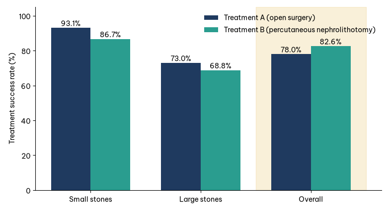
Figure 1 puts the rates from Table 1 side by side: A is higher than B for both stone sizes but lower in the overall column.
2.2. Step 2: the overall rate is a weighted average
Each option's overall rate is the average of its group rates, weighted by each group's share within that option:
Overall rate = Σ (rate in group i × share of group i)
Applied to kidney stones:
A: 93.1% × 25% + 73.0% × 75% ≈ 78.0%
B: 86.7% × 77% + 68.8% × 23% ≈ 82.6%
A puts 75% of its weight on the group with a low baseline rate; B puts 77% of its weight on the group with a high baseline rate. The difference in weights is large enough to swamp A's advantage within each group. This is the common mechanism behind every case of Simpson's paradox in this article.
2.3. Three necessary conditions
The paradox can only occur when all three conditions hold at once:
There is a grouping variable Z (here, stone size).
Z strongly affects the outcome, meaning the groups have clearly different baseline rates.
The distribution of Z differs between the options being compared.
Remove any one condition and the paradox cannot occur. In particular, if two options have the same group composition, their weights are identical and the aggregated figures cannot reverse. Every prevention strategy later in this article builds on this point: make the group composition the same, through study design or statistical adjustment.
3. Simpson's paradox in practice
The same weighting mechanism appears in many fields. The five examples below run from admissions and sports to business and epidemiology, ending with a version for continuous variables.
3.1. Graduate admissions at Berkeley (1973)
For the fall 1973 intake, the University of California, Berkeley was suspected of discriminating against women. The aggregated figures looked stark (Bickel et al., 1975; Table 3):
A 9-percentage-point gap across more than 12,000 applications is unlikely to be chance. But when Bickel and colleagues analysed the data department by department, most departments showed no bias against women; taken across departments, the data even leaned slightly in women's favour.
The explanation lies in where people applied. Women concentrated on highly competitive departments with low admission rates. Men concentrated on easier departments with high admission rates. The overall gap reflects the pattern of field choice, not how each department assessed applications.
The story does not end there. Why did women concentrate in the hardest-to-enter fields? The answer may lie in social factors, education and bias long before anyone applied, a point Bickel and colleagues themselves raised. The department-level analysis shows that admissions committees did not discriminate, but it does not rule out inequality elsewhere. Choosing how to split the data is therefore always an interpretive decision, not a purely technical one.
3.2. Batting averages in baseball
Ross (2004) illustrates the paradox with two players, Derek Jeter and David Justice, over three seasons (Table 4):
Justice beat Jeter in all three seasons, yet combined, Jeter comes out slightly ahead. Weighting is again the reason: 1995 accounted for only about 4% of Jeter's at-bats, so his worst season barely affected his combined figure. For Justice, 1995 accounted for about 39% of his at-bats, and it was also his lowest-scoring season, so his combined figure was dragged down.
3.3. A/B testing in e-commerce
Suppose an online store tests two checkout page designs (illustrative data; Table 5):
On the overall figures, B wins. But on both device types, A has the higher conversion rate. The cause: 80% of A's views came from mobile, compared with 67% of B's, and mobile users buy less to begin with. Choosing B on the overall figure means discarding the better option.
Notably, this is an experiment, not observational data. A warning sign should have been caught early: A received 1,000 views and B received 1,500, whereas an A/B test is usually designed to split traffic evenly. Traffic allocation errors like this can distort results even when randomization is in place (Fabijan et al., 2019; Kohavi et al., 2020).
3.4. COVID-19 case fatality rates
Early in the 2020 pandemic, Italy's case fatality rate (CFR) among recorded cases was higher than China's overall. Yet von Kügelgen and colleagues (2021) showed that when split by age group, Italy's CFR was lower than China's in every age group in the data they compared.
The explanation is the age structure of recorded cases. In Italy, older people made up a much larger share of recorded cases, and this group faces a far higher risk of death. Different testing strategies in the two countries also contributed to the difference.
This example also reveals a subtlety discussed in detail below. The authors did not treat age simply as a confounder, but analysed it as a mediator: country affects who gets infected and tested, and through that, the fatality rate. Which figure is "right" depends on the question being asked. To compare quality of care, you need to compare within age groups or use age-standardized rates, the standard practice in epidemiology when comparing populations.
3.5. A version with continuous variables
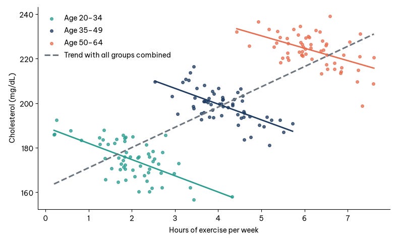
The paradox is not limited to percentages; it also affects correlations between two continuous variables. Consider the relationship between weekly hours of exercise and cholesterol level (hypothetical example):
Across all the data, the trend is upward: people who exercise more seem to have higher cholesterol.
Split by age group, each group shows a downward trend: within the same age, people who exercise more have lower cholesterol.
The reason is that older people both exercise more (on their doctors' advice) and have higher cholesterol because of age. Age is a confounder that tilts the overall trend line upward. Figure 2 illustrates the case with simulated data. This form is easy to spot on a scatter plot coloured by group: each cloud of points slopes downward, but the line joining the centres of the clouds slopes upward.
4. Should you trust the aggregated or the stratified figures?
This is the central question, and the answer is surprising: the data alone cannot answer it. Two datasets can contain identical numbers yet call for opposite readings, depending on the causal structure that generated them. Pearl (2014) clarifies this using causal diagrams; epidemiologists have reached the same conclusion (Hernán et al., 2011).
Let X be the option being compared, Y the outcome, and Z the variable used to split the data. The role of Z determines which figure to read (Table 6).
4.1. Case 1: Z is a confounder
Z affects both the choice of X and the outcome Y. Example: stone size affects which treatment the doctor chooses and the chance of success. Here you should use the stratified figures, or figures adjusted for Z, because Z biases the comparison. The kidney stone and age–cholesterol examples belong to this case.
4.2. Case 2: Z is a mediator
Z lies on the very pathway through which X affects Y. Example: a drug lowers blood pressure, and lower blood pressure reduces the risk of stroke. If you stratify by blood pressure after treatment, you inadvertently block the drug's pathway, and the drug looks useless. If you want the drug's total effect, you should use the aggregated figures.
4.3. Case 3: Z is a collider
Z is affected by both X and Y. Controlling for Z creates a spurious association between X and Y. Example: if you look only at people admitted to a prestigious university, you may find test scores and athletic talent negatively correlated, even though the two are unrelated in the wider population; the university admits people who excel in one or the other. Here too you should use the aggregated figures.
4.4. Bringing the three cases together
The three cases can be condensed into one rule for choosing figures according to the role of Z (Table 7).
The COVID-19 example above shows that the same variable can play different roles depending on the question. The first step is therefore always to state the causal question you want to answer. For more on building and reading causal diagrams, see Greenland et al. (1999) or Pearl et al. (2016).
4.5. A backpack campaign and a causal diagram
Haughton et al. (2026) give a business case that shows what a causal diagram adds when the paradox appears. A company runs an advertising campaign for backpacks. Before the campaign, 2% of customers bought a backpack; six months later the figure is 2.2%, and the marketing department declares success. But split by gender, the purchase rate fell from 4% to 3.5% among men and from 1% to 0.7% among women. The overall rate rose only because the customer mix shifted towards the group that buys more anyway.
The causal diagram for this case has three variables: gender (G), the campaign (C) and backpack sales (S). Gender affects who the campaign reaches (G → C) and the demand for backpacks (G → S); the campaign affects sales (C → S). Gender is therefore a confounder, and the path through G opens a "back door" between the campaign and sales that must be blocked by stratifying or by including gender in the model. Following Case 1 above, the stratified figures are the ones to read, and they suggest the campaign did not work, or at least that there is no evidence it did. One more caveat: this is a before-and-after comparison without a control group, so a general market trend over the six months could also explain the decline.
The example extends into two principles that apply to any regression model. First, a regression coefficient has no causal meaning unless the causal structure behind it is stated. Second, one model measures one effect correctly: in a model with both campaign and gender, the campaign coefficient measures the effect of the campaign, but the gender coefficient in the same model captures only the direct effect of gender, not the part that runs through the campaign. Reading every coefficient in a regression table as a total effect is a mistake common enough that epidemiologists have named it (Westreich & Greenland, 2013). Measuring several effects usually takes several models, each built from the diagram to answer its own question.
When a problem involves dozens of variables, the diagram can be drawn from domain knowledge or estimated from data with structure-learning algorithms. Either way, the conclusion is only credible if the analyst can argue that no important variable has been left out, because an unmeasured confounder still biases the result however elegant the diagram.
5. Prevention through study design
Treat Simpson's paradox as a default risk whenever you compare groups using aggregated figures. The response has three stages: prevention at the design stage, detection during analysis, and correct handling after detection. The first stage is the cheapest, because it breaks the third condition before the paradox can form.
5.1. Randomization
When patients or users are randomly assigned to options, every other variable, including ones nobody has thought of, ends up roughly evenly distributed across groups. The third condition of the paradox is removed.
Had the kidney stone study used randomization, each treatment would have received a share of large stones close to the overall share among all patients, about 49% (343/700), instead of 75% and 23% as actually happened. Only then would comparing the aggregated figures be fair.
Note: randomization only guarantees balance in expectation. With small samples, imbalance can still arise by chance.
5.2. Stratified randomization
If you know an important variable in advance (disease severity, device type, country), randomize separately within each stratum: among large-stone patients, randomly split 50/50 between A and B, and do the same among small-stone patients. This guarantees the same group composition instead of merely hoping for it. In A/B testing, it is equivalent to splitting traffic 50/50 separately for each device type.
5.3. Record all potential confounders
You cannot adjust for a variable you did not measure. Before collecting data, ask domain experts two questions: what makes people choose option A over B, and what else affects the outcome. Then make sure those variables are recorded (Table 8).
5.4. Check for sample ratio mismatch (SRM)
In an A/B test, if the design is a 50/50 split but the actual data come out 53/47, that is a red flag. Technical problems such as bots, page-load errors or caching may be skewing the allocation, and Simpson's paradox may be hiding inside. Fabijan and colleagues (2019) describe sample ratio mismatch (SRM) as one of the most common and serious failures in online experiments.
The usual check is a chi-square test comparing actual counts with expected counts. If the p-value is very small (a threshold of 0.001 is common), find the cause before reading the results (Kohavi et al., 2020).
6. Detection during data analysis
With observational data, there is no randomization to protect you, so the analyst must actively hunt for the paradox. The tools below run from simple to sophisticated.
6.1. Compare group composition first
Before calculating any rate, tabulate the share of each subgroup within each option. In the kidney stone example, the composition table alone (A: 75% hard cases, B: 23% hard cases) is a strong warning sign.
Rule of thumb: if the group composition of two options differs by more than about 10 percentage points on a variable that affects the outcome, treat the aggregated figures as unreliable until you have checked them by group. This is a practical alert threshold, not a statistical standard.
6.2. Stratified analysis
Split the data by each suspect variable and compare again, one variable at a time, then important combinations. The result falls into one of three cases (Table 9):
Distinguishing the last case matters. If A is better for small stones but worse for large ones, the right answer is "it depends on stone size", not "A is better".
6.3. Direct standardization
Standardization brings the options to the same group composition for a fair comparison. For kidney stones, take all 700 patients as the standard population: 357 small-stone cases (87 + 270) and 343 large-stone cases (263 + 80). Then compute the expected successes if each treatment had treated exactly this population (Table 10):
After standardization, the ranking reverses and matches the within-group results. This is the figure to present to the hospital board, alongside the crude figure and an explanation of why the two differ.
6.4. The Mantel–Haenszel odds ratio
For data stratified into several 2×2 tables, the Mantel–Haenszel method computes a single odds ratio (OR) adjusted across strata (Mantel & Haenszel, 1959). For kidney stones, comparing A with B:
Crude OR: about 0.75, so A looks worse than B.
Mantel–Haenszel OR, adjusted for stone size: about 1.45, so A is better than B.
An OR moving from below 1 to above 1 is a quantitative signature of Simpson's paradox. When crude and adjusted estimates differ substantially (many studies use a threshold of about 10%), the variable in question is a suspected confounder. Two cautions apply. First, the OR is non-collapsible: crude and adjusted ORs can differ even without confounding, especially when the outcome is common, as it is here. Second, a common OR is only meaningful when the effect is reasonably homogeneous across strata; the Breslow–Day test helps check this.
6.5. Multivariable regression and the 10% change rule
Regression can adjust for many variables at once, including continuous ones. The screening procedure has three steps:
Fit a model with only the option variable X and record its coefficient.
Add each suspect variable Z to the model in turn.
If X's coefficient changes by more than 10% or changes sign, Z may be a confounder and should be considered for retention.
For kidney stones, in a logistic regression, the coefficient for B versus A is positive in the crude model (B looks better) but negative once stone size is added. The sign change confirms stone size as a confounder.
Caution: the 10% rule is only a screening tool, and it is also affected by the non-collapsibility noted above. Never add a mediator or a collider to a model just because it shifts the coefficient. A variable's causal role must first be established with a causal diagram (Greenland et al., 1999).
6.6. Systematic screening across many variables
With high-dimensional data, repeat the following check for each grouping variable (device, country, channel, age band):
Identify the winning option overall.
Identify the winning option within each group of that variable.
Flag variables where the option winning in every group differs from the overall winner.
The list of flagged variables becomes the priority list for domain experts to review.
6.7. Propensity scores and inverse weighting
When there are too many confounders to stratify by hand, you can use the propensity score: the probability that an individual is assigned to option A, estimated from that individual's characteristics (Rosenbaum & Rubin, 1983). It is used in two main ways:
Matching: for each individual in group A, find the individual in group B with the closest propensity score, then compare outcomes within pairs.
Inverse probability weighting: assign weights so that the two groups have equivalent distributions of characteristics.
After matching or weighting, check the balance of each variable before comparing outcomes; a standardized difference below 0.1 is the usual threshold (Austin, 2011).
Important limitation: these techniques can only adjust for measured variables. To judge how strong an unmeasured variable would need to be to overturn the conclusion, add a sensitivity analysis, such as the E-value (VanderWeele & Ding, 2017).
6.8. Visualization
People spot patterns in pictures faster than in tables of numbers. Three chart types are especially useful:
Grouped bar chart: one cluster of bars per subgroup, with options side by side.
Scatter plot coloured by group, with a regression line for each group and one for all the data. When the group lines slope opposite to the overall line, you are looking at Simpson's paradox.
100% stacked bar chart or mosaic plot: shows the group composition of each option.
7. Handling the paradox once detected
Detecting the paradox is only half the job. The other half has four steps:
Draw a causal diagram to determine whether Z is a confounder, a mediator or a collider. Only when Z is a confounder should stratified or adjusted figures take priority (Pearl, 2014).
Consult domain experts to test the causal assumptions. Statistics cannot replace understanding of the real-world mechanism.
Report both figures, aggregated and stratified (or adjusted), with an explanation of why they differ.
Choose the figure that matches the question. These two questions need two different figures:
This patient has a large stone; which treatment should we use? → the stratified figures.
What overall results does the hospital's current pattern of treatment allocation produce? → the aggregated figures describe this correctly.
7.1. Pitfalls in handling the paradox
Preventing the paradox does not mean slicing the data as finely as possible (Table 11).
7.2. Checklist before trusting an aggregated comparison
Design
☐ Was assignment to options random? If not, who decided, and on what criteria?
☐ Have variables that could affect both the choice of option and the outcome been recorded?
☐ For A/B tests: does the actual allocation match the design (SRM)?
Data
☐ Is the group composition (age, device, region...) comparable across options?
☐ Is any group heavily over-represented in one option?
☐ Does each subgroup have a large enough sample to draw conclusions?
Analysis
☐ Have results been examined within each important subgroup?
☐ Is the direction of the conclusion consistent overall and within each group?
☐ Have crude and adjusted estimates been compared?
☐ Were stratification variables pre-specified to avoid subgroup fishing?
Interpretation
☐ Has the grouping variable been identified as a confounder, mediator or collider?
☐ Have domain experts confirmed the causal assumptions?
☐ Does the report present both aggregated and stratified figures, with an explanation?
☐ Does the chosen figure match the decision question (for an individual or for an overall policy)?
8. Where Simpson's paradox hides in each field
The paradox is not just a textbook curiosity. Almost any field that compares rates across groups with different compositions can run into it (Table 12).
HR (hypothetical example). Company X finds that women's average pay is 8% lower than men's. Split by department, women's pay is equal to or higher than men's within every department; the overall gap comes from women being concentrated in lower-paying departments. The right conclusion is not "there is no problem", but that the problem lies in the allocation of roles, not in pay policy within each department. The remedy is therefore different too, echoing the lesson from Berkeley.
Healthcare. When hospitals are ranked by mortality, tertiary hospitals that receive many severe cases often have higher crude rates even though their care is no worse. That is why serious rankings must adjust for case severity before comparing.
9. Common questions
This section briefly answers six questions that often come up when people first meet Simpson's paradox.
How common is Simpson's paradox?
Complete reversals are relatively rare. Pavlides and Perlman (2009) estimated that for 2×2×2 tables with randomly chosen cell probabilities, the chance of a reversal is only about 1 in 60. But partial distortion, where the conclusion is clearly biased without reversing, is very common in observational data.
Does big data protect against the paradox?
No. The problem lies in the structure of the data, not the amount. The bigger the data, the narrower the confidence intervals, and the more confident we become in a conclusion that may be wrong.
So is it always safe to use the stratified figures?
No. If the grouping variable is a mediator or a collider, stratifying leads to the wrong conclusion (Hernán et al., 2011; Pearl, 2014).
How does Simpson's paradox differ from an interaction effect?
In Simpson's paradox, the direction of the effect is the same in every group but opposite to the overall direction. In an interaction effect, the direction differs between groups, and the right answer is "it depends on the group".
Do randomized experiments eliminate the paradox completely?
Nearly, if they are designed and run correctly, because random allocation makes groups equivalent in expectation. However, technical faults such as SRM can still break randomization, so checks are always needed (Fabijan et al., 2019).
What if I have no data to build a causal diagram?
Causal diagrams are built from domain knowledge, not from data. Sketch a draft with domain experts and refine it over time.
Conclusion
Simpson's paradox is not a flaw in mathematics but a reminder about how people read data. An average can blend many different stories; if we do not separate them, we may reach a conclusion that is the exact opposite of reality. Yet splitting the data mechanically can also mislead. Data do not speak for themselves; our understanding of the process that generated them decides whether we read them correctly (Pearl, 2014).
Three things to remember:
Aggregating data can reverse a trend when the group composition differs between options.
Whether to aggregate or stratify depends on the causal structure and the question being asked, not on the numbers.
Always understand the context behind the data before drawing conclusions.
For managers, this means not making decisions on a single summary metric such as an average KPI or an overall conversion rate. Ask for segment-level figures with an explanation of group composition, and ask "what makes these groups different?" before asking "which option is better?".
The next time you see a report concluding that "X is better than Y", stop and ask: what is this average hiding?
References
Austin, P. C. (2011). An introduction to propensity score methods for reducing the effects of confounding in observational studies. Multivariate Behavioral Research, 46(3), 399–424. https://doi.org/10.1080/00273171.2011.568786
Bickel, P. J., Hammel, E. A., & O'Connell, J. W. (1975). Sex bias in graduate admissions: Data from Berkeley. Science, 187(4175), 398–404. https://doi.org/10.1126/science.187.4175.398
Blyth, C. R. (1972). On Simpson's paradox and the sure-thing principle. Journal of the American Statistical Association, 67(338), 364–366. https://doi.org/10.1080/01621459.1972.10482387
Charig, C. R., Webb, D. R., Payne, S. R., & Wickham, J. E. (1986). Comparison of treatment of renal calculi by open surgery, percutaneous nephrolithotomy, and extracorporeal shockwave lithotripsy. British Medical Journal (Clinical Research Ed.), 292(6524), 879–882. https://doi.org/10.1136/bmj.292.6524.879
Fabijan, A., Gupchup, J., Gupta, S., Omhover, J., Qin, W., Vermeer, L., & Dmitriev, P. (2019). Diagnosing sample ratio mismatch in online controlled experiments: A taxonomy and rules of thumb for practitioners. In Proceedings of the 25th ACM SIGKDD International Conference on Knowledge Discovery & Data Mining (pp. 2156–2164). Association for Computing Machinery. https://doi.org/10.1145/3292500.3330722
Greenland, S., Pearl, J., & Robins, J. M. (1999). Causal diagrams for epidemiologic research. Epidemiology, 10(1), 37–48. https://doi.org/10.1097/00001648-199901000-00008
Haughton, D., Haughton, J., & Lo, V. S. Y. (2026). Cause and effect business analytics and data science. CRC Press.
Hernán, M. A., Clayton, D., & Keiding, N. (2011). The Simpson's paradox unraveled. International Journal of Epidemiology, 40(3), 780–785. https://doi.org/10.1093/ije/dyr041
Julious, S. A., & Mullee, M. A. (1994). Confounding and Simpson's paradox. BMJ, 309(6967), 1480–1481. https://doi.org/10.1136/bmj.309.6967.1480
Kohavi, R., Tang, D., & Xu, Y. (2020). Trustworthy online controlled experiments: A practical guide to A/B testing. Cambridge University Press. https://doi.org/10.1017/9781108653985
Mantel, N., & Haenszel, W. (1959). Statistical aspects of the analysis of data from retrospective studies of disease. Journal of the National Cancer Institute, 22(4), 719–748. https://doi.org/10.1093/jnci/22.4.719
Pavlides, M. G., & Perlman, M. D. (2009). How likely is Simpson's paradox? The American Statistician, 63(3), 226–233. https://doi.org/10.1198/tast.2009.09007
Pearl, J. (2014). Understanding Simpson's paradox. The American Statistician, 68(1), 8–13. https://doi.org/10.1080/00031305.2014.876829
Pearl, J., Glymour, M., & Jewell, N. P. (2016). Causal inference in statistics: A primer. Wiley. https://www.wiley.com/en-us/Causal+Inference+in+Statistics:+A+Primer-p-9781119186847
Pearson, K., Lee, A., & Bramley-Moore, L. (1899). Mathematical contributions to the theory of evolution. VI. Genetic (reproductive) selection: Inheritance of fertility in man, and of fecundity in thoroughbred racehorses. Philosophical Transactions of the Royal Society of London. Series A, 192, 257–330. https://doi.org/10.1098/rsta.1899.0006
Rosenbaum, P. R., & Rubin, D. B. (1983). The central role of the propensity score in observational studies for causal effects. Biometrika, 70(1), 41–55. https://doi.org/10.1093/biomet/70.1.41
Ross, K. (2004). A mathematician at the ballpark: Odds and probabilities for baseball fans. Pi Press. https://www.amazon.com/s?k=A+mathematician+at+the+ballpark+Ross&i=stripbooks
Simpson, E. H. (1951). The interpretation of interaction in contingency tables. Journal of the Royal Statistical Society: Series B (Methodological), 13(2), 238–241. https://doi.org/10.1111/j.2517-6161.1951.tb00088.x
VanderWeele, T. J., & Ding, P. (2017). Sensitivity analysis in observational research: Introducing the E-value. Annals of Internal Medicine, 167(4), 268–274. https://doi.org/10.7326/M16-2607
von Kügelgen, J., Gresele, L., & Schölkopf, B. (2021). Simpson's paradox in COVID-19 case fatality rates: A mediation analysis of age-related causal effects. IEEE Transactions on Artificial Intelligence, 2(1), 18–27. https://doi.org/10.1109/TAI.2021.3073088
Westreich, D., & Greenland, S. (2013). The Table 2 fallacy: Presenting and interpreting confounder and modifier coefficients. American Journal of Epidemiology, 177(4), 292–298. https://doi.org/10.1093/aje/kws412
Yule, G. U. (1903). Notes on the theory of association of attributes in statistics. Biometrika, 2(2), 121–134. https://doi.org/10.1093/biomet/2.2.121