One Analytics Project End to End on a Coffee Chain's Data
Following descriptive, diagnostic, predictive, prescriptive and adaptive analytics through one simulated coffee chain to see how errors travel between stages


Key takeaways
The five types of analytics are most valuable when they form a chain: each stage hands the next one a question, a number or a set of scenarios. An error made early travels all the way to the decision.
In the diagnostic stage, writing down the fingerprint each hypothesis must leave, then testing it with a control group, separated a staffing cut (18.9 percentage points more cancellations) from the manager's favorite suspect, the rain.
The most important choice in the predictive stage is what to predict: forecasting cups sold instead of cups demanded understated midday demand by 11.8% and would have locked in the understaffing.
Because cancellations rise steeply with load, optimizing staff on five demand scenarios beat optimizing on a single point forecast. In an 11-week backtest the first gained about $346 while the second lost about $218.
The final deliverable is not the analysis but a half-page memo: recommendation first, each number with its limits and an answer to the question the reader has not asked yet.
Analytics is usually taught one technique at a time. A course spends a week on dashboards, a week on root-cause analysis, a week on forecasting and a week on optimization, each with its own tidy dataset. That is a reasonable way to learn the tools, but it hides the hardest part of the job: in a real project the five types of analytics do not stand alone. What the descriptive stage finds decides which diagnostic question is worth asking. The mechanism the diagnostic stage uncovers decides what the forecast should predict. The forecast is the input to the prescriptive model. And when the environment changes, the whole chain has to notice and start again.
A chain has a consequence that isolated exercises never show: errors propagate. Suppose the forecasting stage uses "cups sold" as its target instead of "cups customers wanted to buy". The forecast comes out too low. The staffing stage takes that low number, schedules too few people, more customers give up, cups sold fall further and next week's forecast is lower still. No single step looks wrong on its own. The error only becomes visible when you look at the whole chain.
This article walks through one such project end to end, on simulated data from Six Streets, a hypothetical chain of six coffee shops in Ho Chi Minh City that sells over the counter and through food delivery apps. Section 1 introduces the data and a small note-taking tool that keeps the stages connected. Sections 2 to 6 go through the five stages: descriptive, diagnostic, predictive, prescriptive and adaptive. Section 7 shows how the five stages are compressed into a half-page summary for the operations director. The data are simulated on purpose: because we know where the truth lies, we can check whether the methods actually find it.
1. The data and the stage card
This section introduces the Six Streets data and a simple tool that keeps the five stages linked.
The central file has 8,688 rows. The first question to ask of any dataset is what one row represents. Here each row is one shift at one store on one day of 2025: six stores times 362 trading days times four shifts (morning 6 to 10 a.m., midday 10 a.m. to 2 p.m., afternoon 2 to 6 p.m. and evening 6 to 10 p.m.). Each row records the number of staff on the shift, cups sold at the counter, orders placed through the apps and orders canceled. Alongside it come daily weather records and 52,315 individual app orders from one store.
Two columns deserve a careful reading from the start. The app orders column counts every order placed, including those later canceled because the wait was too long, so it measures app demand even when the store cannot keep up. The counter column counts only customers who bought: someone who walks in, sees a long line and walks out leaves no row behind. Counter demand is therefore censored data: we only see the part of demand the store managed to serve. This small detail will decide the fate of the forecasting stage.
To translate operational results into money, the project uses four assumptions: ingredients and packaging cost $0.54 per cup, app prices are 15% higher than counter prices, the apps take a 25% commission on order value and one staff member costs $5.60 for a four-hour shift. At Store 3, where a counter cup sells for $1.80 on average, each counter cup leaves a contribution margin of $1.26 and each app cup about $1.01.
Each stage is recorded on a five-line stage card, a pocket version of the SOAR model (Richardson & Watson, 2024). Table 1 describes the five lines.
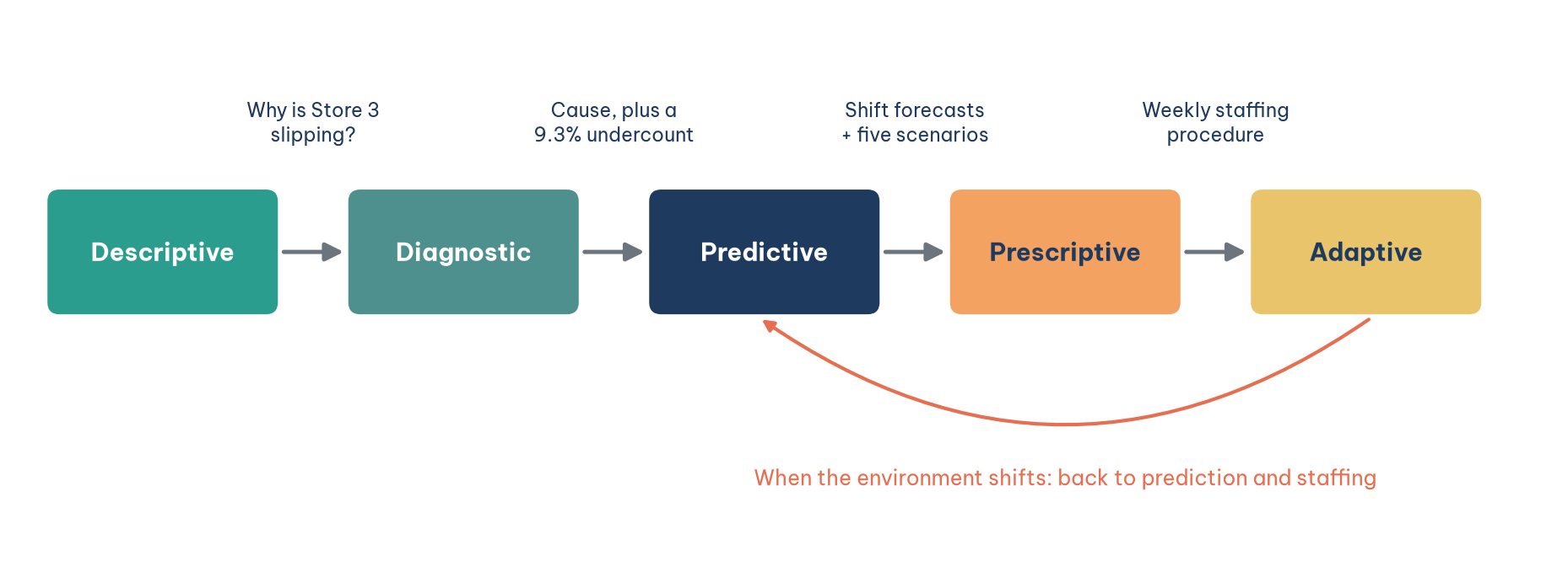
The handoff line is what turns five separate analyses into one project. If you cannot write it, the stage you just finished may be correct but useless. Figure 1 shows the five stages of the project and what passes between them.
2. The descriptive stage: which store is out of step
The first stage answers the question the leadership team asks every month: which store is drifting away from the rest of the chain, and since when?
The most natural comparison is to rank the stores by revenue, and it is also the easiest to get wrong, because the six stores sit in six neighborhoods with different rhythms. Office districts are busy on weekday mornings and lunchtimes, residential districts in the evenings and on weekends. The store near a university follows the academic calendar. Comparing an office store with a residential one compares two different things. The descriptive stage therefore compares each store with itself in an earlier period, using average revenue per trading day and the app cancellation rate.
The result contains three signals. Store 5, near the university, fell 17.4% in July to September compared with the first half of the year, the biggest drop in the chain, but that was the student summer break and it recovered when the semester began. Store 3, in a mixed residential and commercial district, fell only 3.9% from July, from about $1,032 to $991 a day, and was still below its first-half level in the fourth quarter, while its app cancellation rate more than doubled, from 5.2% to 11.7%. Store 4 grew strongly from October (13.9% above its first half) but its cancellation rate rose too, from 5.0% to 13.9%. The most worrying signal was not the largest drop but the small drop that did not recover and came with a deteriorating operational metric. The descriptive stage hands the next stage one question: why has Store 3 been slipping since July? It also leaves an open note about Store 4.
3. The diagnostic stage: why Store 3 is slipping
This section shows how to find a cause when several hypotheses fit the same timing, and how to put a price on the damage.
3.1. Three hypotheses and their fingerprints
The operations director already had an explanation: the 2025 rainy season started in May and June, and customers did not want to go out. Good diagnosis starts by listing several hypotheses before looking at the numbers, because someone who already holds one hypothesis will see every number as evidence for it. Three hypotheses deserve a hearing: rain; lower demand because a competitor opened nearby; and reduced service capacity, because the data show that from 1 July the Store 3 midday shift had three staff instead of four.
All three fit the July timing, so timing cannot decide between them. What can decide is a fingerprint: if a hypothesis is true, it must leave a particular pattern in the data and must not leave certain others. Table 2 writes these fingerprints down before any test is run.
3.2. Four tests
The first test splits Store 3 into its four shifts and compares January to June with July to September, as in Table 3.
The morning, afternoon and evening shifts barely moved. The midday shift changed on every metric, in a chain that reads from left to right: staff fell from four to three; each person had to make more drinks, so load rose from 12.0 to 15.4 cups per hour; preparation time rose by about 70%, from 5.5 to 9.5 minutes; and the cancellation rate almost quadrupled. Meanwhile midday orders placed did not fall at all, edging up from 48.1 to 49.0 a day. Customers kept coming; the store could not serve them in time. That fingerprint rules out lower demand and points straight at service capacity.
The second test separates capacity from rain with a difference in differences: compare the change in the Store 3 midday cancellation rate before and after 1 July with the change at three control stores whose staffing did not change over the same period (Stores 1, 2 and 6; Store 5 is left out because of the summer break and Store 4 to be safe). This is the same logic that Card and Krueger (1994) used to compare fast-food restaurants on either side of a state border after a minimum wage increase. Figure 2 shows the result.
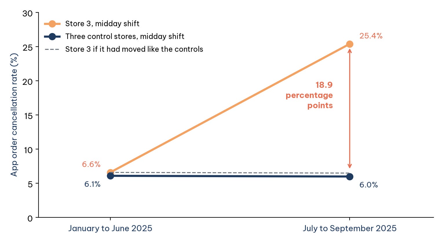
The calculation behind Figure 2 is short: (25.4 − 6.6) − (6.0 − 6.1) = 18.9 percentage points. Rain, if it mattered, would hit both groups alike and is subtracted out; what remains belongs to the one thing only Store 3 experienced, the loss of a midday staff member. The same comparison applied to app orders placed gives a difference of only −1.2%, confirming that app demand did not fall, while counter cups sold at midday show a difference of −9.3%.
The third test answers the director's question with respect: what does rain actually do? Pooling every afternoon and evening shift across the chain by rainfall, days with more than 15 mm of rain had 27.1% fewer counter cups than dry days but 34.0% more app cups, so total demand fell by only 7.0%. Rain mainly switches the channel, in the afternoon and evening, at every store: a completely different fingerprint from the one at Store 3. The fourth test goes down to the 52,315 individual app orders at Store 3 and finds the cancellation rate climbing with waiting time, from 3.2% for orders ready in under five minutes to 67.7% for orders that took more than 14 minutes. That is exactly the mechanism of understaffing.
Put together, the diagnostic stage concludes that Store 3 slipped because its midday shift lost a staff member on 1 July. From July to December the extra cancellations cost 2,746 app cups (about $2,780 of contribution margin) and the shortfall at the counter cost another 1,989 cups (about $2,508). That is roughly $201 a week, several times the cost of one more person on seven midday shifts, about $39 a week. The stage hands on two things: the question "how busy will each shift be next week?" and a warning that midday counter demand is being undercounted by about 9.3%, because customers who walk away leave no trace.
4. The predictive stage: how much demand each shift will face
To rebuild the schedule we need to know how busy each shift will be next week. This section shows that the most important decision in the forecasting stage is not choosing a model but choosing what to forecast.
The natural target is cups sold, because that is the number already in the reports. But midday cups sold at Store 3 have already been cut by the shortage of staff. With the same model, switching the target from cups demanded to cups sold lowers the midday forecast by 11.8%, while the other shifts move by only about 2%. A schedule built on that lower forecast would understaff again, which is exactly the self-reinforcing loop described at the start. The project therefore forecasts cups demanded: counter cups plus app cups ordered, including canceled orders, and then scales up the midday counter component to correct for the 9.3% undercount handed over by the diagnostic stage (a factor of 1/(1 − 0.093), about 1.10).
Three models are compared, from crude to refined. Model A takes the value for the same weekday and shift last week. Model B averages the same weekday and shift over the last four weeks. Model C pools the five weekdays into one group, Saturday into a second and Sunday into a third, then averages the last eight weeks of that group for the same shift. The pooling is justified by the data: in the first half of the year the busiest weekday was only 3.9% above the quietest. The models are scored by rolling-origin evaluation: stand at each past week, use only data available before that week to forecast it, then compare with what actually happened (Hyndman & Athanasopoulos, 2021). Table 4 shows the results over 17 weeks, from 1 September to 28 December 2025.
Model C wins, with a MAPE of 8.9% against 11.8% for Model A, and the reason it wins matters more than the number. Model A rests on one observation, so it carries all of last week's noise into next week: one rainy day last week becomes a low forecast this week. Model C rests on about forty observations for a weekday, so the noise cancels out. Pooling similar days beats chasing the most recent week. Even so, the best model is still off by about 9% on average. Rather than hide that error, the project records it as a distribution: in 80% of weeks, actual demand fell between 0.87 and 1.18 times the forecast. Cutting that distribution at its 10th, 30th, 50th, 70th and 90th percentiles gives five demand scenarios, at 0.866, 0.964, 1.015, 1.065 and 1.179 times the forecast. That set of scenarios, not a single number, is what passes to the next stage.
5. The prescriptive stage: how many people to schedule on each shift
With demand forecasts in hand, the next question is a decision. This section links the forecast to action in three steps: a curve, a marginal calculation and an optimization model.
The first step is to estimate a cancellation curve by load from all 8,688 shifts in the chain: how the share of app orders canceled rises as the number of cups each staff member must make per hour goes up. The curve is a logistic function of the queueing term u/(1 − u), where u is load divided by an assumed working capacity of 20 cups per person per hour; this form captures waiting times that grow slowly while the counter has slack and explode as it approaches full capacity. Figure 3 shows how sharply it bends.
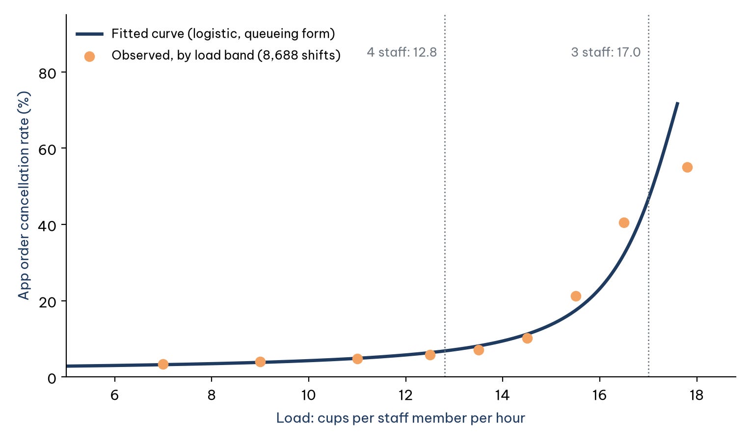
Take the midday shift on Monday 5 January 2026, with a corrected demand forecast of 205 cups. With three staff the load is 17.0 cups per person per hour and the expected cancellation rate is 55.5%. That sounds extreme, but it is consistent with the data: in December 2025 the Store 3 midday shift already had a cancellation rate of 36.8% at an average load of 16.1. With a fourth person the load falls to 12.8 and the expected cancellation rate to 8.1%.
The second step is marginal value: how much contribution margin each additional person brings in, compared with the $5.60 wage for a shift. The rule is simple: keep adding people while the gain exceeds the wage. The gain shrinks quickly. On that Monday morning, with demand of 176 cups, the third person adds about $47, the fourth about $13 and the fifth about $1. At midday the fourth person adds about $43 and the fifth about $3, so four is the right number. In the evening, a third person would add about $1.21 and is not worth scheduling. The third step is integer programming for the whole week: when total staff-shifts are limited, the 28 cells of shift and day compete for a shared resource, and the model chooses a staffing level for each cell to maximize total contribution margin minus wages.
One design decision is the easiest to overlook: in what form should demand enter the model? Because the cancellation curve bends so sharply, forecast errors have asymmetric effects. A day 15% busier than forecast pushes a shift onto the steep part of the curve and loses many orders, while a day 15% quieter only leaves a few staff with spare time. The 55.5% above already shows this: read off the curve at the average load alone, the midday cancellation rate with three staff would be about 50%, but averaged over the five scenarios it is 55.5%, because the busy scenarios land where the curve is steepest. Optimizing on the average ignores this asymmetry and tends to understaff, a pattern Savage (2009) calls the flaw of averages. Table 5 compares the options for the week of 5 January, each evaluated over the five scenarios.
Optimizing on the point forecast trims staff to 82 shifts and leaves almost twice as many canceled cups as the scenario-based schedule. The scenario-based schedule adds a fourth person to the midday shift every day and cuts the weekend morning shift to three people. Expected contribution margin minus wages rises by about $244 a week, and expected canceled cups fall from 384 to 114.
6. The adaptive stage: when the environment changes and nobody says so
Every number in the prescriptive stage assumes that next week looks like the past eight weeks. This section asks what happens when that assumption breaks: does the system notice by itself?
The open note from the descriptive stage returns here. From October 2025, weekday morning and midday demand at Store 4 jumped for a reason the data do not record (in the simulation, a new office building opened next door). A slow eight-week average keeps forecasting too low for weeks: the model fitted once at the end of September and used unchanged underestimated weekday morning and midday demand by 40% to 54% every week from early October. The adaptive stage compares three forecasting strategies and adds a break alert: when a shift's forecast error exceeds 15% in the same direction two weeks in a row, the system treats it as a structural break, discards the data before the break and re-estimates from the new data only. In the simulation the alert fired on 13 October for the morning shift (33.1% off for the second week running) and on 20 October for the midday shift (22.2%). Over 12 weeks from 6 October, this rule cut the MAPE of weekday morning and midday forecasts at Store 4 from 30.8% with the static model (and 11.9% with plain weekly re-estimation) to 7.8%. It relied only on the forecast errors themselves; nobody had to report the new building.
The last check matters more: does a better forecast become a better decision? Replaying the whole chain of forecasting and staffing against actual demand over 11 weeks from 13 October, the scenario-based schedule earned about $346 more than the old schedule, while a schedule optimized on point forecasts lost about $218, with 2,834 canceled cups against 2,126 under the old schedule and 1,567 under the scenario-based one. Same forecast, two ways of using it, two results of opposite sign. For the week of 5 January the proposed Store 4 schedule adds a person to weekday morning and midday shifts and is expected to raise contribution margin minus wages by about $111 a week.
This stage also produces a set of operating rules that divide work between machine and people: the system forecasts and proposes a schedule every week; the store manager approves it; and break alerts go to the area manager, who looks for the cause before the system re-estimates. Table 6 condenses the five stages onto one page.
7. From five stage cards to half a page for the director
Five stage cards are the analyst's notebook, not a report for the decision maker. This section shows how they are compressed into an executive summary.
Three principles govern the summary. First, the recommendation comes first, not the analytical journey. Second, every recommendation carries a number and the limits of that number. Third, the summary answers the question the reader has not asked but will, here "what about the rain?", because a question left unanswered comes back in the meeting and casts doubt on everything else. The summary sent to the Six Streets operations director has five short paragraphs:
Recommendation. From the week of 5 January 2026, hire a replacement midday staff member for Store 3 and reduce the Store 3 weekend morning shift to three people; at the same time, adopt the new Store 4 schedule with an extra person on weekday morning and midday shifts.
Why. Store 3 has slipped since 1 July because its midday shift lost a staff member: midday app cancellations rose 18.9 percentage points more than at the comparison stores, while orders placed did not fall. The estimated loss is about $201 a week, several times the cost of one more person ($39 a week). The proposed Store 3 schedule raises expected contribution margin minus wages by about $244 a week; the new Store 4 schedule by about $111 a week.
About the rain. Rain does reduce counter customers, but they switch to ordering through the apps; total demand falls only a few percent, in the afternoon and evening at every store. Rain does not explain what happened at Store 3.
What could be wrong. The benefits are model-based estimates; the staffing model ignores counter customers who walk away, so it most likely understates the benefit. The system will track forecast error every week and flag any shift that misses by more than 15% two weeks in a row.
Decision needed. Approve the hire by Wednesday 31 December 2025 so that it is in place for the week of 5 January.
The summary is shorter than a page, carries only a handful of key numbers and contains no jargon such as "difference in differences" or "integer programming". Those things are still there, in the appendix and the five stage cards, for anyone who wants to check. The reader of the summary needs to be able to trust the conclusion; the reader of the appendix needs to be able to verify it.
Conclusion
The Six Streets project shows that the five types of analytics are worth most when they are linked into a chain. The descriptive stage picked the right signal: a small decline that did not recover, not a large seasonal one. The diagnostic stage used fingerprints and a control group to separate the real cause from the explanation everyone already believed. The predictive stage chose the right thing to forecast before choosing a model. The prescriptive stage respected the asymmetry of risk instead of optimizing on an average. The adaptive stage turned the whole chain into a system that notices when the world changes.
The lesson that runs through the project lies in the joints. The 9.3% undercount traveled from diagnosis to forecasting; the five scenarios traveled from forecasting to staffing; and in the final check, the same forecast produced results of opposite sign depending on how it was used. An analytics project is not judged by how sophisticated each stage is, but by whether the final decision is better, and by whether the decision maker can trust the conclusion and verify it.
References
Card, D., & Krueger, A. B. (1994). Minimum wages and employment: A case study of the fast-food industry in New Jersey and Pennsylvania. American Economic Review, 84(4), 772–793. https://www.jstor.org/stable/2118030
Hyndman, R. J., & Athanasopoulos, G. (2021). Forecasting: Principles and practice (3rd ed.). OTexts. https://otexts.com/fpp3/
Richardson, V. J., & Watson, M. W. (2024). Introduction to business analytics. McGraw Hill. https://www.mheducation.com/highered/product/introduction-business-analytics-richardson-watson/9781265450175.html
Savage, S. L. (2009). The flaw of averages: Why we underestimate risk in the face of uncertainty. Wiley. https://www.oreilly.com/library/view/the-flaw-of/9780470488126/
Discussion about this post