How Recommender Systems Get to Know You
How shopping sites and streaming apps turn your clicks, purchases and viewing history into a guess about what you will want next


Key takeaways
Recommender systems grew in layers: association rules find items bought together, collaborative filtering learns from people with similar histories and matrix factorization discovers hidden "taste dimensions".
A rule with high confidence can still be useless. Lift, which compares a rule with the item's normal popularity, shows whether buying one item really changes the chance of buying another.
Almost every technique can be seen as link prediction: guessing a missing edge between a user and an item in a large graph.
Modern platforms run a multi-stage pipeline (candidate generation, ranking, re-ranking) on implicit feedback in near real time, often within a few hundred milliseconds.
Offline accuracy is not the goal. Real systems are judged by A/B tests, diversity and fairness as well, because optimizing clicks alone can trap users in filter bubbles and bury small sellers.
Have you ever wondered how Netflix seems to know the next film you want to watch, or how Amazon suggests a product you did not yet realize you needed? It is not magic. It is one of the most successful and widespread applications of data science: the recommender system.
These invisible machines work quietly behind the digital platforms people use every day, shaping what they see and steering what they choose. Their reach is enormous. According to two Netflix product leaders, about 80% of the hours streamed on the service come from recommendations, and personalization saves the company more than $1 billion a year by keeping subscribers from leaving (Gomez-Uribe & Hunt, 2015). Users of YouTube, TikTok, Spotify, Amazon or regional marketplaces such as Shopee in Southeast Asia meet recommender systems many times a day, usually without noticing.
This article peels back the layers of a recommender system, from the simplest principles to complex techniques, and shows how they relate to one another. Section 1 starts with the oldest technique: finding items that are often bought together. Section 2 turns to collaborative filtering, the approach that made Netflix famous, with a small worked example. Section 3 steps back to view every technique as a link prediction problem on a graph. Section 4 introduces content-based filtering and hybrid systems. Section 5 describes how modern recommender systems work at scale, Section 6 discusses how to evaluate them, Section 7 offers practical notes for smaller businesses and Section 8 brings all the techniques together in one table.
1. The starting point: items bought together
This section explains the oldest recommendation technique and the three measures used to judge its rules.
Start with the simplest scenario: a grocery store wants to arrange its shelves to sell more. It analyzes thousands of receipts to see which products are often bought together. This is the essence of co-occurrence grouping, also called frequent itemset mining or association rule mining.
1.1. Association rules and three measures
The core idea is to find patterns in how often products appear in the same basket. Suppose the data show that 70% of customers who buy beer and ice also buy peanuts. That produces a rule: if {Beer, Ice} then {Peanuts}.
Is that 70% enough to trust the rule? To answer, analysts use three measures for a rule {A} → {B}:
Support: the share of all receipts that contain both A and B. A rule with very low support may be a coincidence, or it may not be worth acting on because too few customers are involved.
Confidence: among receipts that contain A, the share that also contain B. The 70% above is the confidence.
Lift: confidence divided by the overall share of receipts that contain B. A lift above 1 means buying A makes buying B more likely than usual; a lift close to 1 means the two purchases are almost independent.
Table 1 shows why lift matters, using 1,000 hypothetical receipts.
The two rules in Table 1 have the same support and confidence. Yet rule 2 says nothing: 70% of beer-and-ice buyers also buy bottled water, exactly the same share as all customers. Rule 1, in contrast, shows that beer-and-ice buyers are almost three times as likely as usual to buy peanuts. An analyst who looks only at confidence would rate the two rules equally; lift reveals which pair is worth placing side by side.
The best-known application of this technique is Amazon's "Frequently bought together" feature. The system does not need to know who you are; it relies only on the history of millions of transactions.
1.2. The algorithms: Apriori and FP-Growth
Finding association rules among millions of transactions requires efficient algorithms, and two are used most often.
Apriori (Agrawal & Srikant, 1994) rests on a simple but powerful principle: if a set of items is frequent, every subset of it must also be frequent. Put the other way round, if {Beer} is already rare, there is no need to examine {Beer, Ice, Peanuts}. The algorithm scans the data several times and drops infrequent sets as it goes, which saves it from checking billions of combinations.
FP-Growth (frequent pattern growth; Han et al., 2000) is a more efficient improvement. Instead of scanning the data many times, it compresses the whole transaction database into a compact tree structure called an FP-tree and mines frequent patterns directly from that tree, which cuts computing time considerably.
The approach works well, but it has one major limitation: it is not personalized. Every customer who buys beer and ice gets the same suggestion, whoever they are. Getting past that limit required the next step in the evolution.
2. Collaborative filtering: learning from people like you
This section covers the technique that made Netflix famous, in its three main branches, with a small calculation to show how similarity is measured.
Instead of looking only at products, collaborative filtering (CF) puts users and the community at the center. Its core assumption is that people who behaved similarly in the past will have similar tastes in the future.
2.1. User-based collaborative filtering
This method looks for your "data twins": the users most like you. It then recommends what they liked. It works in two steps: find the users whose ratings, viewing or purchase history most resembles yours, then recommend items they liked that you have not yet touched.
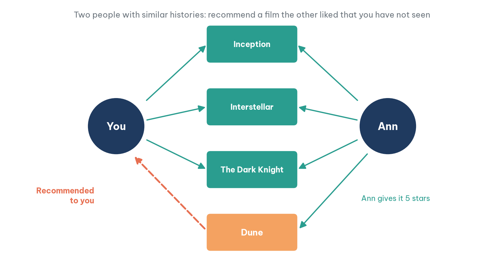
For example, you and Ann both love Inception, Interstellar and The Dark Knight. Ann recently watched Dune and gave it five stars. The system notices how similar you and Ann are, and because you have not seen Dune, it recommends the film to you. Figure 1 illustrates the mechanism.
The key question is how to measure "similar". Consider a small worked example. Table 2 shows the ratings (on a 1 to 5 scale) that four users gave to five films; an empty cell means the user has not seen the film.
The most common measure is cosine similarity: treat each person's ratings as a vector and measure the angle between two vectors, using only the films both have rated. Table 3 shows the results, together with a second measure that first subtracts each person's average rating (equivalent here to the Pearson correlation coefficient).
Table 3 holds three practical lessons. First, cosine on raw ratings can mislead. Ben's taste is the opposite of yours, yet the cosine is 0.59, because all ratings are positive and so every vector points in roughly the same direction. Subtracting each person's average before comparing (to see which films they like more than their own usual level) gives a truer answer: −0.97, almost perfectly opposite. Second, similarity based on little shared data is unreliable. Cara's cosine is 0.99, but it rests on just two films; after subtracting means it cannot be computed at all, because you rated both of those films 5 and your ratings do not vary. Real systems usually shrink the weight of pairs with few items in common. Third, this shortage of shared data is the main weakness of the method when a catalog holds millions of items and each person has rated only a few dozen.
Your predicted rating for Dune can then be calculated. Your most similar user is Ann (0.87). Ann rated Dune 5, which is 0.8 points above her average of 4.2 across her five ratings. Your average across the four films you have rated is 3.75. The prediction is 3.75 + 0.8 = 4.55, or about 4.6, high enough to recommend.
2.2. Item-based collaborative filtering
Instead of comparing users, this method compares items directly. The system builds a similarity matrix between items, based on how strongly the same users rate or choose them. When you like item A, it recommends the items B, C and D that are most similar to A.
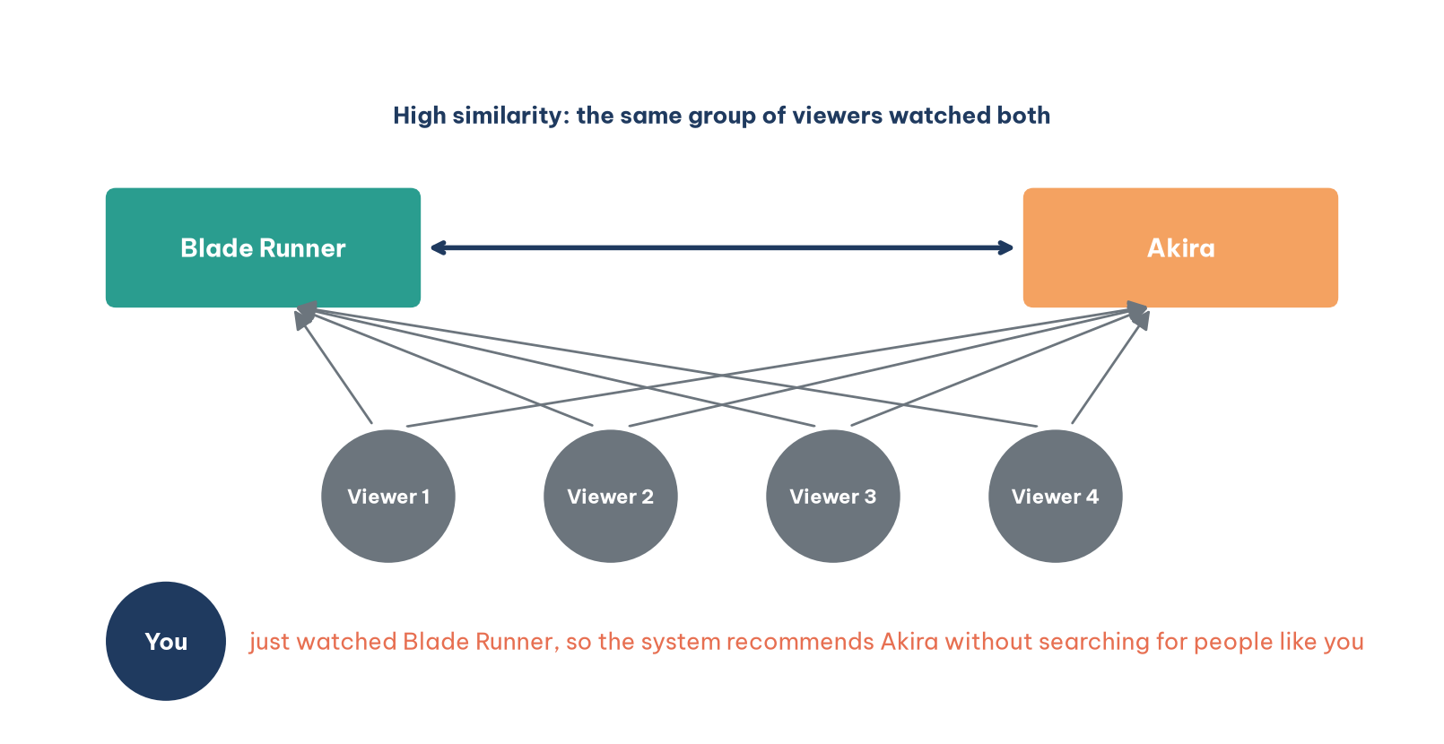
For example, the system notices that most people who watched Blade Runner also watched Akira. When you finish Blade Runner, it recommends Akira, as Figure 2 shows.
Amazon pioneered this technique at scale (Linden et al., 2003). The reason is that it is more stable and scales better: relationships between items change far more slowly than one person's tastes, so the item similarity matrix can be computed in advance on a schedule and looked up very quickly when a user arrives. Item-based recommendations are also easier to explain: "because you watched Blade Runner" is a reason any user understands at once.
2.3. Model-based collaborative filtering: matrix factorization
The two methods above are memory-based: they work directly on historical data. The real breakthrough came from model-based methods, above all matrix factorization, the foundation of the winning entries in the Netflix Prize (2006 to 2009). In that competition, Netflix offered $1 million to any team that could improve the accuracy of its Cinematch rating predictions by 10%.
The problem. Instead of only knowing that you liked films A and B, can a system learn why you liked them? Perhaps you enjoy films with intricate plots, or films with subtle humor. These traits are called latent information, because no column in the data records them.
The solution. Matrix factorization reduces the dimensions of the data to discover these hidden taste spaces.
Input: a huge user-film matrix, with millions of users and thousands of films, in which each cell is a rating. Almost all cells are empty, just like your Dune cell in Table 2 but on a vastly larger scale.
Process: the algorithm factors this matrix into two smaller ones. A user-factor matrix represents each person as a vector of preferences along hidden dimensions, such as how much they like action or romance. An item-factor matrix represents each film as a vector of traits along the same dimensions.
Result: users and films are projected into the same multidimensional taste space. A person's predicted rating for a film is approximately the dot product of the two vectors. To make recommendations, the system looks for films whose vectors best match the user's vector.
A visual example. Koren et al. (2009), members of the team that won the Netflix Prize, plotted the first two latent dimensions found in the competition data. Figure 3 redraws part of their illustration.
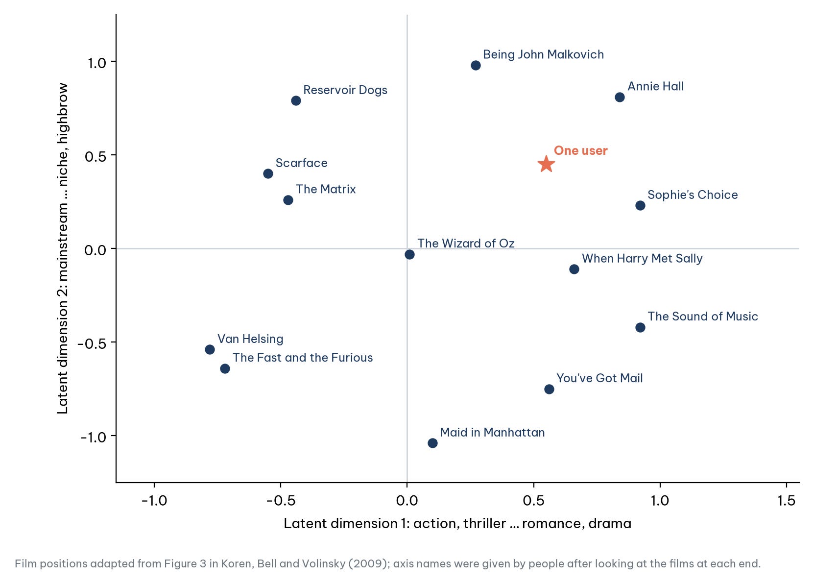
In Figure 3, the horizontal axis separates action and thriller films on the left (Van Helsing, The Fast and the Furious) from romance and drama on the right (The Sound of Music, Sophie's Choice). The vertical axis separates niche, highbrow films at the top (Being John Malkovich, Annie Hall) from mainstream entertainment at the bottom (Maid in Manhattan, You've Got Mail). A user is placed in the same space according to their viewing history, and the films near that position are good candidates to recommend.
An important caveat: the algorithm does not "know" the names of the axes. People look at the films at the two ends of each axis and then name it. The first two dimensions are often easy to interpret; many other latent dimensions are much harder to read, even though they still make predictions more accurate.
A revealing detail about the Netflix Prize. Netflix never put the full winning solution into production. According to the Netflix technology blog, two of its main algorithms (matrix factorization and a type of neural network) were adopted, but the extra gain from blending hundreds of models was not worth the engineering cost. Moreover, once Netflix moved to streaming, the most important data were no longer star ratings but actual viewing behavior (Amatriain & Basilico, 2012). The lesson: accuracy on a test set is not always what a business needs most.
So far there are three techniques that look rather different: association rules look at items, collaborative filtering looks at users and matrix factorization finds a hidden space. Is there a way to see them as one problem?
3. A general lens: recommendation as link prediction
This section steps back and treats users, items and interactions as one large network, which turns recommendation into the problem of predicting missing links.
3.1. The core idea
In a network (graph) made of nodes and links, link prediction estimates how likely a missing link is to exist or to form in the future (Liben-Nowell & Kleinberg, 2007). Link prediction is not a single technique but a framework that generalizes recommendation problems:
Co-occurrence grouping is link prediction on an item graph. Nodes are items; a link joins two items that are often bought together. The task: when a user views node A, predict its likely links to other nodes.
Collaborative filtering is link prediction on a user-item graph. Nodes are users and items (a bipartite graph); a link is an interaction such as a purchase, a view or a like. The task: predict a missing link between a user node and an item node.
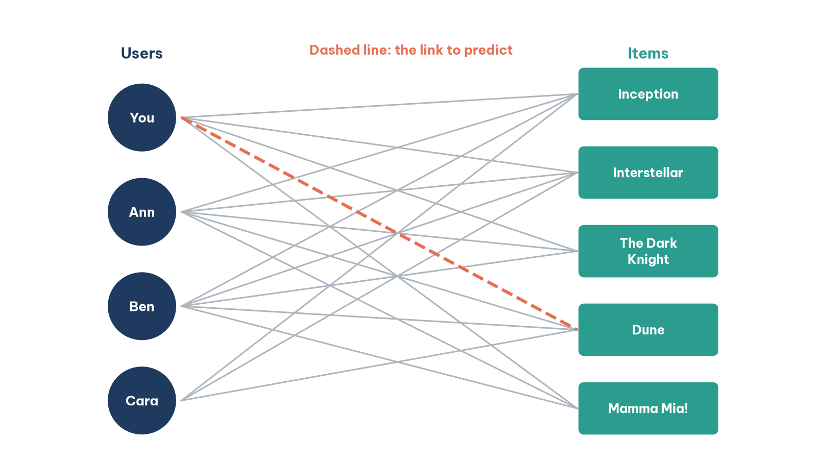
Figure 4 draws the data of Table 2 as a bipartite graph. The question "should the system recommend Dune to You?" becomes "should there be an edge between You and Dune?".
Link prediction is used far beyond products and films. It powers "People you may know" on Facebook and LinkedIn, predicts interactions between proteins in biology to support disease research and flags accounts that are likely to be connected within a fraud network.
3.2. Three approaches
Data scientists have developed three main families of methods for this problem.
Similarity-based heuristics. This is the most intuitive approach: use measures of graph structure to score pairs of nodes that are not yet linked.
Common neighbors: count the neighbors two nodes share. Two people with many mutual friends on Facebook probably know each other.
Jaccard coefficient: a normalized version of common neighbors, equal to the number of shared neighbors divided by the total number of distinct neighbors of the two nodes.
Adamic-Adar index (Adamic & Adar, 2003): a subtler measure that treats a "rare" shared neighbor (one with few connections) as more informative than a "popular" one. Each shared neighbor contributes 1/ln(number of that neighbor's connections). Suppose two people share two contacts: a specialist with 3 connections contributes 1/ln 3 ≈ 0.91, while a celebrity with 50 connections contributes only 1/ln 50 ≈ 0.26. Both knowing someone who keeps a small circle means far more than both following a celebrity.
Predictive modeling. This approach turns link prediction into a familiar binary classification problem: for each unlinked pair of nodes, predict whether a link exists (1) or not (0). The neat twist is that the model's features are the similarity measures above (common neighbors, Adamic-Adar and so on), plus node attributes such as a user's age, location or school. These features feed logistic regression, random forests or gradient boosting.
Graph-based methods. This is the most modern and powerful family, using the whole structure of the graph.
Random walks: algorithms such as PageRank and Personalized PageRank simulate a "random walker" moving around the graph. If a walker starting from node A often visits node B, a link between A and B is likely.
Graph embeddings and graph neural networks: these learn to represent each node as a vector of real numbers (an embedding) so that nodes close together in the graph have similar vectors. Link prediction then becomes a search for nearby vectors in the embedding space.
The key point that ties this section back to Section 2: matrix factorization is itself a form of graph embedding for the bipartite user-item graph. The user and film vectors in Figure 3 are embeddings of the nodes in Figure 4.
All of these techniques depend on interaction history. What happens with a brand-new item that nobody has bought or watched yet?
4. Content-based filtering and hybrid systems
Collaborative filtering relies on other users' behavior, so it struggles when an item or a user is new. This section introduces a complementary approach based on the item's own attributes and then shows how large platforms combine several techniques in a hybrid system.
4.1. Content-based filtering
Content-based filtering recommends items based on their intrinsic attributes: genre, cast, director, description, price, brand. If you listen to U2, the system looks for bands with similar characteristics, such as The Killers. It does not need data from other users.
Its biggest advantage is that it addresses the cold start problem. A film released today has no viewers yet, so collaborative filtering does not know whom to recommend it to, but content-based filtering still knows it is a science fiction film starring a particular actor. Its drawback is a tendency to recommend "more of the same", rarely helping users discover something new.
4.2. Hybrid systems
In practice, almost no system relies on a single technique. Large platforms use hybrid systems that combine the strengths of several methods. Netflix, for example, might use content-based filtering to recommend a film that has just been released, collaborative filtering (matrix factorization) to personalize more deeply based on your taste space and co-occurrence grouping to fill a "Because other viewers also watched" row. Each row on the home page may come from a different algorithm.
How these techniques are assembled at the scale of billions of users is the subject of the next section.
5. What a modern recommender system looks like
This section describes the multi-stage architecture that large platforms use today and the three ways they differ from the Netflix Prize era.
Large platforms such as YouTube, TikTok, Spotify or Shopee still build on the ideas above, but they organize them into a multi-stage pipeline that can handle billions of items within a few hundred milliseconds (Covington et al., 2016). Figure 5 shows the pipeline.
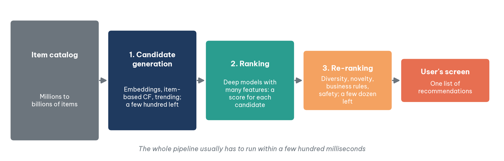
Table 4 describes the job of each stage and the techniques typically used.
The reason for splitting the work into stages is a trade-off between speed and accuracy. Stage 1 must be extremely fast, so it uses simple calculations on embeddings; stage 2 handles only a few hundred candidates, so it can afford complex models with many features. The techniques from Sections 1 to 4 therefore do not disappear: they become "candidate sources" in stage 1.
Compared with the Netflix Prize era, modern systems differ in three major ways.
Implicit feedback instead of ratings. Users rarely give star ratings, but their behavior always leaves traces: watch time, scrolling past, clicks, adding to cart, rewatching. These data are called implicit feedback. They are far more plentiful but also harder to interpret: scrolling past a video may mean dislike, or simply that the user was busy.
Near real-time updates. TikTok's recommender is known for reacting to the few videos you have just watched within minutes, instead of waiting for a daily retraining. ByteDance has described part of an architecture that allows such continuous model updates (Liu et al., 2022).
Balancing exploitation and exploration. If a system recommends only what it is sure you will like, it never learns what else you might like. So part of the recommendations is set aside to try new things, accepting the risk that you will not like them in exchange for more information.
From 2024 to 2026, large language models began to appear in recommender systems: reading product descriptions and text reviews, explaining why something is recommended or letting users "chat" their way to a product. Yet candidate generation and ranking at scale still rely mainly on embeddings and specialized deep learning models, because of speed and cost requirements.
How is such a complex system evaluated? The answer goes well beyond "what percentage of predictions were correct".
6. Evaluating recommender systems: beyond accuracy
This section shows why a single accuracy number is not enough and which other groups of measures real systems need.
The Netflix Prize measured success with one number: the error in predicted ratings. Real systems need several groups of measures, as Table 5 shows.
The first two groups often conflict with the last two. A system that optimizes only click-through rate can push users into a filter bubble: they see only content similar to what they already liked, or content that grows ever more sensational because sensational content gets clicked. On e-commerce marketplaces, popularity bias means best-selling products get recommended still more, while small sellers with good products but few sales struggle to be seen, a self-reinforcing loop.
Regulation has begun to address these problems. In the European Union, the Digital Services Act requires every online platform to explain in plain language the main parameters of its recommender systems, and it requires very large online platforms to offer at least one option for each recommender system that is not based on profiling (European Parliament & Council of the European Union, 2022). Designing a recommender system is therefore a business and ethical problem, not only an algorithmic one.
7. Practical notes for smaller businesses
Most examples in this article come from global platforms with hundreds of millions of users. This section shows how a small or medium business, such as an online bookstore, a cosmetics chain or a language-learning app, can start much more simply.
Start with association rules and item-based collaborative filtering. With a few tens of thousands of orders, the techniques in Section 1 and Section 2.2 are enough to build valuable "frequently bought together" and "customers also viewed" sections. They are easy to deploy and easy to explain, and they need no complex infrastructure. Popular e-commerce platforms and sales management tools often include these features out of the box.
Use lift, not just confidence. As Table 1 showed, a rule with high confidence can be meaningless if the right-hand item is already common. In a store where shopping bags or bottled water appear on almost every receipt, ignoring lift will produce a flood of useless "discoveries".
Measure with A/B tests, not only offline accuracy. A model that predicts historical data better will not necessarily raise revenue. The only way to know is to split customers at random into two groups, one seeing the new recommendations and one seeing the old, and then compare the results.
Respect data protection rules. A personalized recommender system processes personal data. Data protection laws in many jurisdictions, such as the European Union's General Data Protection Regulation, generally require a business to state the purpose of processing and to have a lawful basis for it. A sensible practice is to say clearly in the privacy policy that behavioral data are used to recommend products and to let users switch personalization off.
8. The big picture
This section brings the techniques discussed above together in one place. Table 6 summarizes them.
Conclusion
The history of recommender systems is an impressive evolution: from finding general patterns in transaction data, to modeling the "wisdom of the crowd", to capturing people's hidden, abstract tastes through mathematical models. Seen through the lens of link prediction, all these techniques share one goal: finding valuable connections in a sea of data.
Yet the stories of the Netflix Prize, of filter bubbles and of popularity bias also show something else: the best technique on a leaderboard is not necessarily the best system for a business, and the system best optimized for clicks is not necessarily the best for its users. The next time a recommendation feels exactly right, remember that behind it lies a combination of statistics, graph theory and machine learning, as well as human choices about what the system should optimize.
References
Adamic, L. A., & Adar, E. (2003). Friends and neighbors on the Web. Social Networks, 25(3), 211–230. https://doi.org/10.1016/S0378-8733(03)00009-100009-1)
Agrawal, R., & Srikant, R. (1994). Fast algorithms for mining association rules. In Proceedings of the 20th International Conference on Very Large Data Bases (pp. 487–499). https://www.vldb.org/conf/1994/P487.PDF
Amatriain, X., & Basilico, J. (2012, April 6). Netflix recommendations: Beyond the 5 stars (Part 1). Netflix Technology Blog. https://netflixtechblog.com/netflix-recommendations-beyond-the-5-stars-part-1-55838468f429
Covington, P., Adams, J., & Sargin, E. (2016). Deep neural networks for YouTube recommendations. In Proceedings of the 10th ACM Conference on Recommender Systems (pp. 191–198). https://doi.org/10.1145/2959100.2959190
European Parliament & Council of the European Union. (2022). Regulation (EU) 2022/2065 of the European Parliament and of the Council of 19 October 2022 on a Single Market for Digital Services and amending Directive 2000/31/EC (Digital Services Act). Official Journal of the European Union, L 277, 1–102. https://eur-lex.europa.eu/eli/reg/2022/2065/oj
Gomez-Uribe, C. A., & Hunt, N. (2015). The Netflix recommender system: Algorithms, business value, and innovation. ACM Transactions on Management Information Systems, 6(4), Article 13. https://doi.org/10.1145/2843948
Han, J., Pei, J., & Yin, Y. (2000). Mining frequent patterns without candidate generation. In Proceedings of the 2000 ACM SIGMOD International Conference on Management of Data (pp. 1–12). https://doi.org/10.1145/342009.335372
Koren, Y., Bell, R., & Volinsky, C. (2009). Matrix factorization techniques for recommender systems. Computer, 42(8), 30–37. https://doi.org/10.1109/MC.2009.263
Liben-Nowell, D., & Kleinberg, J. (2007). The link-prediction problem for social networks. Journal of the American Society for Information Science and Technology, 58(7), 1019–1031. https://doi.org/10.1002/asi.20591
Linden, G., Smith, B., & York, J. (2003). Amazon.com recommendations: Item-to-item collaborative filtering. IEEE Internet Computing, 7(1), 76–80. https://doi.org/10.1109/MIC.2003.1167344
Liu, Z., Zou, L., Zou, X., Wang, C., Zhang, B., Tang, D., Zhu, B., Zhu, Y., Wu, P., Wang, K., & Cheng, Y. (2022). Monolith: Real time recommendation system with collisionless embedding table. arXiv. https://arxiv.org/abs/2209.07663
Discussion about this post