Finding Causality in Data: RCTs, A/B Tests and Natural Experiments
How to tell whether a change really caused a result: randomized trials, A/B testing, and the quasi-experiments that work when you cannot run an experiment


Key takeaways
Correlation is not causation: a confounder can drive both the "cause" and the "effect".
Randomized controlled trials balance even the factors you cannot measure, which is why they are the gold standard; A/B testing is their fast, cheap digital version.
Experiments on people have ethical limits, and online experiments often run without users' knowledge, so companies must set their own boundaries.
When you cannot randomize, six quasi-experimental methods (natural experiments, instrumental variables, propensity score matching, difference-in-differences, regression discontinuity, synthetic control) look for hidden randomness, each resting on an assumption you must check.
Different methods can give very different answers on the same data, so choose by the data and the question, and report more than one estimate.
The core question is always the same: does my comparison group really show what would have happened without the change?
Have you ever wondered how scientists can say with confidence that a new vaccine will save millions of lives? Or how technology companies such as Google and Amazon know whether a small change to an interface really increases revenue?
The answer lies not in a CEO's genius intuition or a veteran professor's hunch. It lies in experimental thinking.
This article has six parts. Section 1 clarifies the difference between correlation and causation, and why confounding variables make observational data so misleading. Section 2 introduces the "gold standard", the randomized controlled trial (RCT), and Section 3 its pragmatic digital version, A/B testing. Section 4 discusses the ethical limits of experiments on people. Section 5 presents six methods for causal inference when experiments are impossible, with the assumption behind each. Section 6 summarizes how to choose a method for your question and your data, with a more detailed flowchart for business settings.
1. Correlation and causation
Before reaching for these powerful tools, we have to get past a classic thinking trap, one that catches even the smartest minds: confusing correlation with causation.
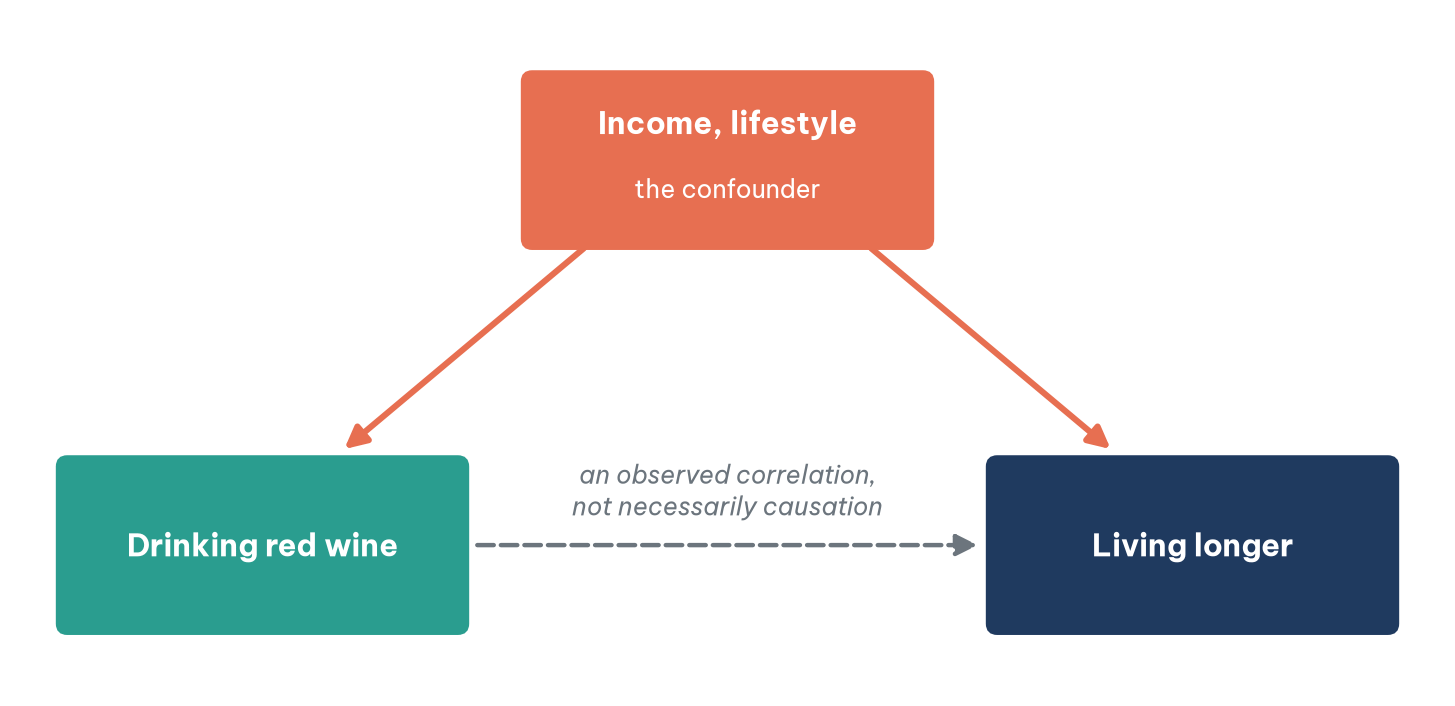
Imagine reading a health statistic: "People who drink a lot of red wine tend to live longer." Your brain immediately urges you to conclude that red wine is an elixir of long life (causation).
But the truth behind the data may be quite different. People who regularly enjoy red wine tend to be middle or upper class. They have higher incomes, healthier diets, exercise regularly and have access to the best healthcare. Here, drinking wine and living longer simply go together (correlation). The real driver, the root cause, is income and lifestyle.
In data science, this income factor is called a confounding variable, or confounder, a trap for unwary analysts. Figure 1 illustrates the structure: the confounder acts on both the "cause" and the "effect", creating a correlation that is easily misread as causation.
So the question is: how do we see through the fog of correlation? How do we control for confounders to find a reliable causal relationship?
That is where the randomized controlled trial (RCT) comes in.
2. RCTs: the scientific gold standard
The randomized controlled trial has long been regarded as the pinnacle of scientific evidence. Its mechanism is elegant but extraordinarily powerful at tying down confounders: you take a set of participants and split them into two groups completely at random. One group receives the intervention (the treatment group); the other receives nothing or a placebo (the control group).
Because group assignment is decided by chance, every characteristic of the participants, from age, sex and income to genes and daily habits, is spread evenly across both sides. The deck is dealt fairly. If outcomes differ between the groups by more than chance can explain (checked statistically), we have strong grounds to conclude that the difference is the causal effect of the intervention. Randomization balances even the factors we do not know about and cannot measure; no other method has that power. But it does not eliminate chance error entirely, so samples must be large enough and results should be replicated.
2.1. The Salk polio vaccine trial (1954)
To appreciate the power of RCTs, go back to the United States in 1954. Polio was a terror at the time, killing and paralysing tens of thousands of children every year. Dr Jonas Salk had developed a promising vaccine, but how could he prove it was effective and safe before mass vaccination?
The 1954 field trial, funded by the National Foundation for Infantile Paralysis, involved about 1.8 million children. Of these, about 600,000 were in the placebo-controlled part: randomly assigned, half received the vaccine and half an inactive solution (a placebo); the rest followed a less rigorous "observed control" design. Crucially, the trial was double-blind: neither the doctors giving the injections nor the parents knew whether a child received the real vaccine or saline. This removed the psychological bias of those assessing the results.
The result? The vaccinated group had a much lower rate of disease. In 1955 the results were announced and the Salk vaccine was licensed the same day. It was the randomized, placebo-controlled part that provided the most convincing evidence. The Salk vaccine, and later Sabin's oral vaccine, helped nearly eliminate polio from most of the world.
2.2. RCTs in business and management
If RCTs once stayed mostly in medical laboratories, today the power of random assignment guides billions of dollars of decisions and helps companies and governments reshape how they operate:
People analytics: instead of arguing about policies, companies use RCTs to measure effects. One example is instructive precisely because it is not an RCT: in 2019, Microsoft Japan gave all its staff Fridays off in August and reported that sales per employee rose about 40% on the same period a year earlier. With no randomly chosen control group, the figure may reflect seasonality, new products or a "being watched" effect; a causal conclusion needs a tighter design. Real RCTs are used to test whether a training programme actually raises productivity, or whether those who signed up were simply already high performers (removing the confounder of personal motivation).
Public policy and government: the UK government's Behavioural Insights Team (the "Nudge Unit") tested tax-reminder letters written in different styles for randomly selected groups of taxpayers. Group A received a stern letter threatening penalties; group B received a letter appealing to social norms ("9 out of 10 people in your area have paid their tax"). The trials found that letters citing social norms raised on-time payment; by the team's own estimate, the changes brought in hundreds of millions of pounds earlier.
Finance and poverty reduction: economists who went on to win the 2019 Nobel Prize used RCTs to test ways of fighting poverty. Abhijit Banerjee, Esther Duflo and Michael Kremer used RCTs to test programmes such as microcredit, deworming pupils and incentives for vaccination. For example, when neighbourhoods in Hyderabad, India, were randomly chosen for new microfinance branches, the effects on income and spending were much smaller than popularly expected at the time (Banerjee et al., 2015). RCTs help base policy on evidence rather than belief.
Operations and supply chains: a large logistics company can test a new delivery-routing algorithm by applying it to a randomly selected half of its trucks while the other half keep the old algorithm. The RCT shows whether the new algorithm really saves fuel and delivery time before it is rolled out to a fleet of tens of thousands.
Pricing and retail: randomly offering different prices or subscription plans to offline customer groups helps find the profit-maximizing price without hurting purchase rates. Supermarket chains often pick 50 stores at random to test a new layout (for example moving the bakery near the entrance so the smell encourages buying) and compare their sales with 50 control stores that keep the old layout.
Strategic meaning: at the top level, RCTs have one vital purpose: reducing the risk of huge investments. Changing an HR policy or redesigning a supply chain costs millions of dollars. RCTs help leadership move from a culture of gut feeling, the HiPPO culture (Highest Paid Person's Opinion), to evidence-based management. Experimental evidence outranks personal opinion, even that of the most senior person. But real-world RCTs are often expensive and slow. The digital environment has created a much faster and cheaper version.
3. A/B testing: the pragmatic RCT of the digital age
If an RCT is like a careful medical professor bound by strict ethical rules, A/B testing is a young Silicon Valley "growth hacker": fast, pragmatic and obsessed with speed.
Mathematically, an A/B test is an RCT simplified and automated for the internet. Instead of randomly assigning patients to test a drug, engineers randomly split a website's or app's traffic into two groups: group A sees the current interface (control), group B sees a slightly changed interface (variant). The goal is not some deep scientific truth but a very practical question: "Which version makes more money?".
3.1. Google's "41 shades of blue" (2009)
One of the best-known examples of A/B testing took place at Google in 2009. The design team could not agree on which blue to use for ad links on the search results page. Instead of endless meetings driven by personal taste, Marissa Mayer (then a product executive) ordered A/B tests of... 41 different shades of blue.
Google's systems randomly split tens of millions of users, with each small group seeing only one shade. The system quietly recorded the click-through rate (CTR) of each colour. The winner was a slightly purplish blue with the highest click rate. According to Dan Cobley, then Google's UK marketing director, the change brought in about USD 200 million a year in extra ad revenue. The story is also controversial: Douglas Bowman, a designer who left Google in 2009, criticized the approach for turning design into choosing between tiny variations rather than generating new ideas. A/B testing proved a blunt truth: in business, you do not need to explain why users like that blue; you only need data showing that they really do, with their clicks.
3.2. A/B testing in business and management
In the digital world, where the cost of running a test is close to zero, A/B testing is the lifeblood of every growth strategy:
E-commerce: sites such as Amazon optimize the checkout flow by repeatedly testing a single-page checkout against a multi-page one. They also test the position, colour and size of the "Add to cart" button and different recommendation algorithms to see which design gets customers to buy fastest.
Content personalization: Netflix is a master of this. For the same series, Stranger Things, user A (who watches horror) sees eerie artwork, while user B (who watches romance) sees romantic artwork. The algorithm continually tests thousands of thumbnails and titles to choose the version that keeps users on the platform longest.
Product development and SaaS: software companies constantly test the experience for new users. Group A gets a feature-limited free tier (freemium), group B a full-featured 14-day trial, to see which brings in more paying customers. They also test onboarding with a three-minute video against interactive step-by-step pop-ups (gamification) to measure retention.
Digital marketing: A/B testing is marketers' bread and butter. They send the same email content with two different subject lines to random customer groups to see which gets the higher open rate. They test ad images that appeal to emotion (fear, joy) against images that appeal to reason (features, price) to optimize cost per click.
Pricing strategy: testing the anchoring effect on a pricing page. Group A sees plans from low to high price; group B sees them from high to low, with the middle plan highlighted as "Most popular". The A/B test shows which order yields the highest average revenue per user (ARPU). The line between "good presentation" and "manipulation" needs careful thought (see the ethics section below).
Strategic meaning: if RCTs help avoid costly macro mistakes, the value of A/B testing lies in the compounding effect. A small change found through A/B testing may lift conversion by only 1%. But if every week you find a genuine 1% improvement, after a year the improvements add up to a large number. A caution: many A/B "wins" are false positives from testing too many variants or stopping tests too early; companies with strong experimentation cultures (Microsoft, Booking.com) report that most ideas tested do not improve the metric (Kohavi et al., 2020). Beyond that, A/B testing creates a culture of "fail fast, fail cheap". Any employee with a new idea can put it to an A/B test and check it with real data, instead of writing long presentations to persuade their bosses. The truth belongs to customers, and customers vote with their clicks.
4. Ethical limits: when experiments cross a red line
The continuity between the medical laboratory (RCTs) and the digital world (A/B testing) is sometimes blocked by an invisible but vital wall: research ethics.
In medicine or psychology, to run an RCT you must pass strict review by an ethics committee (an institutional review board, IRB). You must show the trial does no harm, explain the risks clearly and, above all, obtain participants' written informed consent. On the internet, however, billions of users are "guinea pigs" in thousands of A/B tests every day without knowing it.
4.1. The "Monster Study" (1939): a lesson from psychological research
To understand why RCTs are bound by ethics, look at history. In 1939, under the supervision of psychologist Wendell Johnson, graduate student Mary Tudor experimented on 22 orphans in Iowa. A group of children who spoke normally were repeatedly told they stuttered and criticized for how they spoke. Many in this group became anxious and reluctant to speak; some later described lasting harm. In 2007 the state of Iowa paid compensation to former participants. It is one of the cases that led to ethical rules for research on human beings.
4.2. Facebook's emotional contagion experiment (2014)
In the digital age, however, this line has been blurred. In 2014 Facebook published a scientific paper that caused an uproar. For one week in 2012, it had adjusted the News Feed of nearly 690,000 users without telling them: one group saw fewer positive posts, another fewer negative posts. The aim was to test whether "emotions spread through social networks" (Kramer et al., 2014). The result was yes, though the effect was very small: people who saw fewer positive posts used slightly fewer positive words. Facebook immediately faced a huge wave of anger. Manipulating the moods of hundreds of thousands of people without consent was a serious breach of the line between "product optimization" (A/B testing) and "psychological experimentation on human beings" (RCTs).
4.3. Other red lines
It is not only Facebook. Corporate hunger for optimization through A/B testing and RCTs regularly collides with ethical and legal barriers:
Price discrimination: in 2000, Amazon secretly tested different prices for the same DVD for different customers to measure price elasticity (customers using different browsers saw different prices). When customers found out, Amazon apologized, refunded the differences and promised not to test prices that way again.
Influencing political behaviour: in 2010, Facebook ran an experiment on 61 million users on the day of the U.S. congressional elections. One group saw an "I Voted" button with photos of friends who had voted; the other did not. The authors estimated that the message, directly and through friends, added about 340,000 votes (Bond et al., 2012). The chilling question scholars raised: what if an algorithm showed the button only to supporters of one party?
Exploiting gig workers: ride-hailing apps such as Uber were exposed for repeatedly testing psychologically manipulative interfaces (dark patterns), such as sending "You're so close to your goal, just $10 more" notifications just as a driver was about to log off. The aim was to make drivers work longer, benefiting the platform more than the drivers.
Medical algorithms and clinical equipoise: suppose a health-tech company develops an AI that predicts suicide risk extremely accurately. To prove its effectiveness with an RCT, it would have to give doctors in group A the alerts and deliberately withhold them in group B to see whether death rates differ. In medical ethics, deliberately withholding a potentially life-saving tool just to collect research data is absolutely forbidden.
5. When you cannot experiment: causal inference from observational data
These ethical barriers pose a hard problem: what do you do when you want to understand causation, but ethics (or cost) rules out random assignment?
How do you prove that going to university really leads to higher pay? You cannot toss a coin and force 5,000 pupils to leave school and work while forcing another 5,000 into university. How do you know smoking causes cancer? You cannot make a group of healthy people smoke two packs a day for 20 years. How do you know whether violent films make children more aggressive? You certainly cannot lock a group of children in a room and make them watch violent films every day. Questions like these are everywhere: does a popular crime drama encourage real-life gangs? Does more education cause higher wages, or do the same abilities drive both?
No ethics committee would allow such experiments. When RCTs are ruled out, data scientists and economists turn to a subtler art: causal inference with observational data through quasi-experiments. Instead of creating randomness themselves, they look for randomness hidden in real life. The six methods below are the most common; each rests on its own assumption, and Table 1 at the end of the section summarizes them.
5.1. Natural experiments
A natural experiment occurs when a random event in life, nature or macro policy happens to split people into "treatment" and "control" groups, like an RCT created by nature.
Case study: the U.S. draft lottery (1969). How did serving in the Vietnam War affect a young American man's later income? You cannot randomly force one man into the army and let another stay home. But in 1969 the U.S. government did exactly that, through a lottery of birth dates. Men whose birthdays drew low numbers were drafted; those with high numbers stayed home. This created a great natural experiment. By comparing tax data decades later, economist Joshua Angrist (1990) found that in the early 1980s, white veterans earned about 15% less than men who had not been drafted, reflecting the economic cost of losing years of civilian work experience.
5.2. Instrumental variables
When you see that people with university degrees earn more, you cannot immediately conclude that the degree is the reason. They may have been more able, or had a better family springboard, to begin with (confounders). To solve this without forcing anyone out of school, economists use instrumental variables (IV): a factor that affects schooling but is essentially random and unrelated to ability or family background.
Case study: month of birth and earnings (Nobel Prize in Economics 2021). Angrist and Alan Krueger (1991) noticed that compulsory schooling laws in many U.S. states required children to stay in school until age 16, while school entry depended on year of birth. This created a "natural experiment": children born in December started school earlier than children born in January. When both reached their 16th birthday (the age they could legally leave), the December child had completed about a year more schooling than the January child. Month of birth is essentially random and unrelated to ability, yet it forced one group to stay in school longer than another. By comparing the later earnings of people born in January and December, Angrist and Krueger estimated that each extra year of (legally compelled) schooling raised earnings by about 7–8%. They estimated causation without an experiment. The method has also been criticized: Bound et al. (1995) showed that when the instrument has only a weak effect on schooling (month of birth changes schooling by only a few months), the estimate can be biased. Angrist shared the 2021 Nobel Prize in Economics with David Card and Guido Imbens for contributions to causal inference methods.
5.3. Propensity score matching (PSM): finding "twins" in the data
Return to the question: do violent films make children more aggressive? Observational data may show that children who watch violent films fight more. But perhaps those children live in homes with little parental attention, which makes them both more exposed to violent films and more prone to aggression. Films may be just a "symptom".
Here researchers use propensity score matching (PSM). The logic of PSM is: if you could not randomize from the start, look for "twins" in the data you already have.
An application: an algorithm calculates a "propensity score" for each child from dozens of characteristics: parents' income, mother's education, hours parents spend playing with the child, neighbourhood and so on. It then pairs child A (who watches violent films) with child B (who does not), provided they have nearly identical propensity scores (similar family backgrounds and parental attention). By discarding children with no "twin" and comparing only well-matched pairs, researchers create a simulated RCT. If child A still behaves more aggressively than child B, that is stronger evidence for the role of violent films. An important limit: PSM balances only the factors that are measured and included in the model. If an important factor is unmeasured (for example a child's innate temperament), the conclusion can still be wrong. That is the core difference from an RCT.
Three things are easy to overlook when PSM is used in practice. The first is common support: compare only cases whose propensity scores fall in the range where both groups are present. A child with a score of 0.95 and no comparable child in the other group must be dropped, and the price is that the conclusion holds only for the range of scores that remains. The second is checking balance: after matching, the two groups must be similar on each measured characteristic, not just on the overall score; two people with a score of 0.65 can still be a 70-year-old retired man and a 30-year-old lawyer. The third is the choice of matching variant: there are many ways to match (nearest neighbour, caliper, kernel weighting), and analysts are tempted to try several and report only the most "sensible" result. King and Nielsen (2019) go further, showing that the more balanced the original data, the more propensity score matching can degrade the estimate, and argue that propensity scores should not be used for matching at all.
Recent practice has therefore moved towards two other uses of the propensity score (Haughton et al., 2026). Inverse probability weighting (IPW) drops no one but weights every case: a treated person who was unlikely to be treated gets a large weight, because they "stand in" for many similar people who were not treated, much like weights in a sample survey. When scores are close to 0 or 1 the weights become very large and the estimate unstable, so stabilised or trimmed weights are commonly used. Doubly robust estimation combines regression with inverse weights: as long as one of the two models (the outcome regression or the propensity score model) is correctly specified, the estimate remains reliable. One lesson from an illustration in the book is worth remembering: on the same data about an honours programme, the estimated effect on student retention is 0 with PSM, 0.11 with regression adjustment and 0.25 with coarsened exact matching. The choice of method genuinely changes the conclusion, so a good report presents several estimates and explains why one was chosen as the main result.
5.4. Difference-in-differences (DiD)
Sometimes a new policy is introduced in one area but not another. That is a golden opportunity for difference-in-differences. It does not just compare two groups; it compares how each changed over time (before and after the event).
An application: suppose state X suddenly bans the sale of violent video games to minors, while neighbouring state Y does not. How do you know whether the ban reduced youth crime? Comparing crime in X and Y after the ban would be misleading, because the two states already had different crime levels. DiD solves this by:
calculating the change in crime in state X, before versus after the ban;
calculating the change in crime in state Y over the same period;
subtracting state Y's change from state X's change.
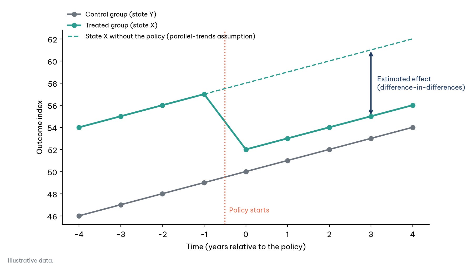
If crime in state X falls sharply while state Y keeps its old trend, the researcher removes factors that affected both states (such as a recession) and has grounds to believe the ban reduced crime. The key condition is the parallel-trends assumption: without the ban, crime in the two states would have changed along the same trend. The usual check is whether the two states' trends were parallel for several years before the policy. A classic example is Card and Krueger's (1994) study of a minimum-wage increase in New Jersey compared with neighbouring Pennsylvania.
Figure 2 illustrates the logic: the dashed line is "state X without the policy", constructed by assuming state X would have moved in parallel with state Y; the gap between the actual line and the dashed line is the estimated effect.
5.5. Regression discontinuity design (RDD): exploiting hard cut-offs
Life is full of rigidly drawn lines. Regression discontinuity design exploits that rigidity to find causation by comparing people just on either side of the line.
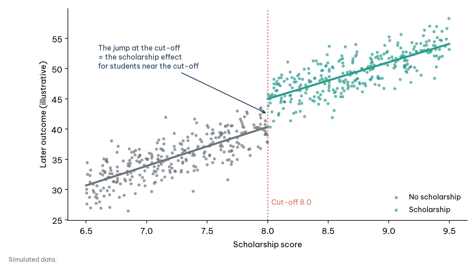
An application: does receiving a university scholarship help students succeed later? You cannot award scholarships at random. Suppose the cut-off score for a scholarship is 8.0. Compare students who scored 7.9 (just missed) with those who scored 8.0 (just made it). In ability and effort, the two groups are almost identical (a 0.1-point gap is more luck than anything). The only difference is that one side gets the money. The cut-off creates an almost randomized situation (Thistlethwaite & Campbell, 1960) for measuring the scholarship's effect, but only for students near the cut-off; it says nothing about students scoring 6 or 9.5. The method also requires that no one can "adjust" their score to cross the threshold. Figure 3 shows the idea: if the scholarship has an effect, the outcome line will "jump" exactly at the cut-off.
5.6. Synthetic control: building a "parallel universe"
This is the most advanced method for when only ONE unit is affected (for example one country changes a law) and no other unit is similar enough to serve as a control. The solution is to use an algorithm to build a "synthetic" unit from the data of many others.
Case study: California's Proposition 99 (1988). In 1988, California passed Proposition 99, raising the tobacco tax by 25 cents a pack and using the proceeds for anti-smoking programmes. How do you know whether it really reduced smoking? Researchers could not find another state identical to California. Instead, Abadie et al. (2010) used an algorithm to weight other states to "assemble" a synthetic California that best matched the real California before 1988: about 39% Utah, 23% Nevada, 20% Montana, 16% Colorado and 7% Connecticut. It is a "parallel universe" in which Proposition 99 never existed. By comparing real and synthetic California, they estimated that by 2000, cigarette consumption in California was about 26 packs per person per year lower than it would have been without the law.
Table 1 summarizes the six methods, their key assumptions and the classic example of each.
6. Which method fits your question?
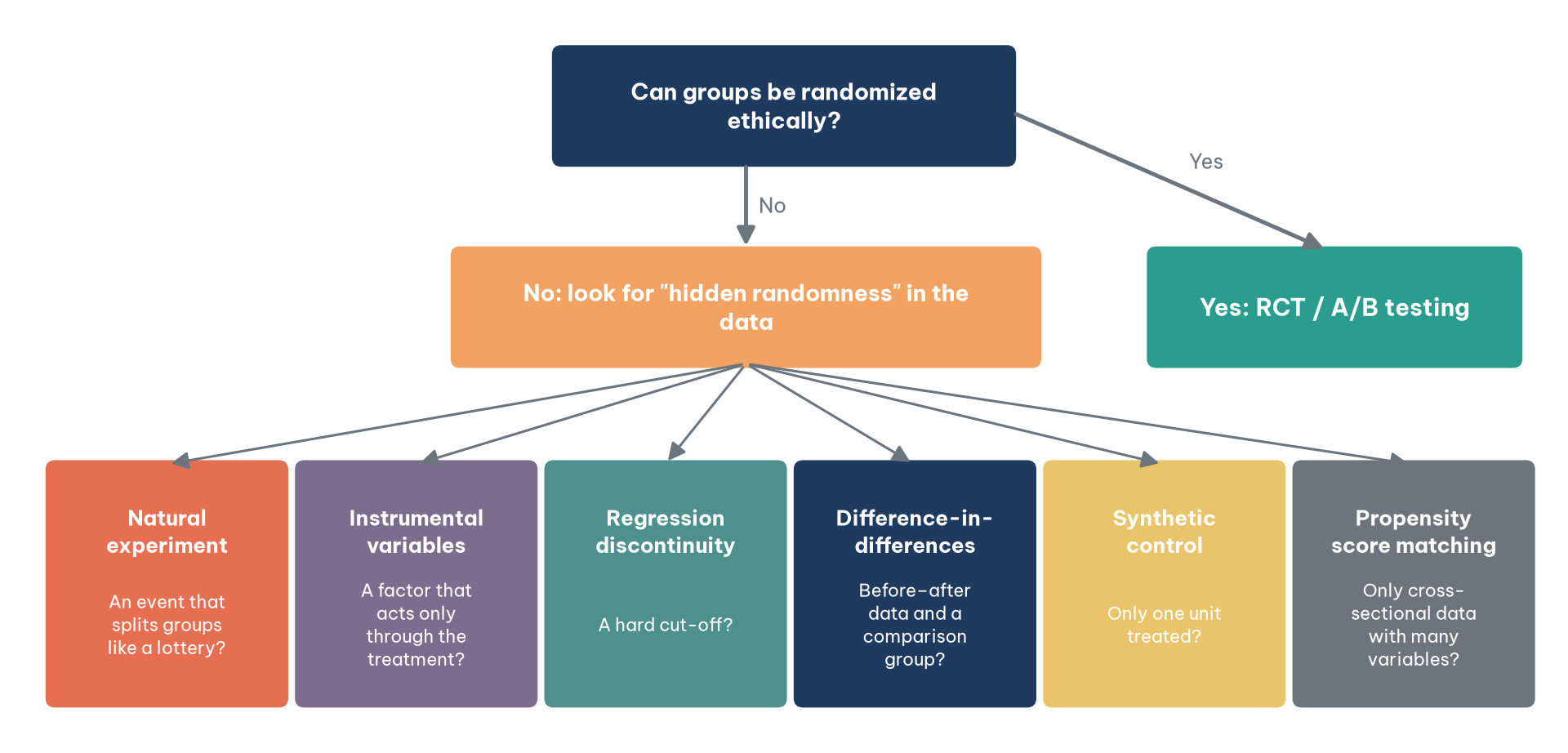
With six quasi-experimental methods plus RCTs and A/B testing, the practical question is where to start. Figure 4 proposes a simple decision tree. The first question is always whether groups can be randomized ethically and feasibly; if so, that is the strongest option. If not, look at the structure of your data and situation to find "hidden randomness": an event like a lottery, a hard cut-off, a policy applied in one place but not another.
Many real situations have the structure of these methods. Minimum wages that differ by region and change over time suggest a difference-in-differences design across regions. University admission cut-offs, scholarship thresholds and company-size thresholds for tax incentives are hard cut-offs suited to regression discontinuity. Pilot policies tested in some provinces or cities before being scaled up create opportunities for difference-in-differences or synthetic control; Vietnam, for instance, often pilots policies in a few provinces before rolling them out nationally. Inside companies, a promotion run in only some stores, or a process change introduced from a particular date, can be evaluated in the same way, provided the analyst checks the assumptions carefully. Table 2 compares the three broad approaches in this article.
The decision tree in Figure 4 is enough to get started. For business problems in more depth, Haughton et al. (2026) propose a more detailed flowchart with two notable features. First, the experimental branch has several options too: if only one variable is tested (say, price), an A/B test is enough, or an A/B/n test when there are several levels; if several variables are tested at once (interest rate, annual fee and benefits of a credit card), a multivariate test with a full or fractional factorial design avoids running dozens of separate A/B tests.
Second, with observational data the first question is whether there is a clear causal hypothesis. If you already know what effect you want to measure on what, you are asking about the "effects of causes", for example how much demand changes when the price changes. If you do not yet know which variables are causes and which are outcomes, you are also asking about the "causes of effects", for example which of many customer interactions (opening an email, visiting the website, browsing a product) leads to a cross-sale. Questions of the second kind require drawing or estimating a causal diagram before measuring anything. Table 3 summarizes the branches of the flowchart.
Table 3 is a reminder that the choice of method starts from the data you have and the question you are asking, not from the method you are used to. A team that only knows regression will see every problem as a regression problem, while a hard cut-off in a customer policy or a rollout staggered across branches may offer much stronger evidence.
Conclusion
The search for causation is challenging but fascinating. Whether you are a scientist looking for a new treatment, a marketer trying to grow sales or a policymaker, experimental thinking remains the most reliable compass. This article has moved from the trap of correlation, through RCTs and A/B testing, to the ethical limits and six methods for observational data. What they all share is one question: does my comparison group really tell me what would have happened without the intervention? Randomization answers it most strongly; the other methods answer it through assumptions that need checking. With observational data, the same question can yield three different numbers depending on the method, so compare several estimates and report the ones that disappoint as well.
Do not let important decisions in your business or project depend on gut feeling or endless meetings driven by the opinion of the highest-paid person (HiPPO). Experimental thinking, the habit of asking "what would have happened without this change?", works at every scale.
If you are developing a new feature in an app, set up a small A/B test. If you are researching a large-scale solution, design a rigorous RCT. And if ethics does not allow that, remember that observational data always hold "natural experiments" waiting to be discovered. Every method rests on assumptions; a good analyst knows the assumptions of the method they use and checks them.
References
Abadie, A., Diamond, A., & Hainmueller, J. (2010). Synthetic control methods for comparative case studies: Estimating the effect of California's tobacco control program. Journal of the American Statistical Association, 105(490), 493–505. https://doi.org/10.1198/jasa.2009.ap08746
Angrist, J. D. (1990). Lifetime earnings and the Vietnam era draft lottery. American Economic Review, 80(3), 313–336. https://www.jstor.org/stable/2006669
Angrist, J. D., & Krueger, A. B. (1991). Does compulsory school attendance affect schooling and earnings? Quarterly Journal of Economics, 106(4), 979–1014. https://doi.org/10.2307/2937954
Banerjee, A., Duflo, E., Glennerster, R., & Kinnan, C. (2015). The miracle of microfinance? Evidence from a randomized evaluation. American Economic Journal: Applied Economics, 7(1), 22–53. https://doi.org/10.1257/app.20130533
Bond, R. M., Fariss, C. J., Jones, J. J., Kramer, A. D. I., Marlow, C., Settle, J. E., & Fowler, J. H. (2012). A 61-million-person experiment in social influence and political mobilization. Nature, 489, 295–298. https://doi.org/10.1038/nature11421
Bound, J., Jaeger, D. A., & Baker, R. M. (1995). Problems with instrumental variables estimation when the correlation between the instruments and the endogenous explanatory variable is weak. Journal of the American Statistical Association, 90(430), 443–450. https://doi.org/10.1080/01621459.1995.10476536
Card, D., & Krueger, A. B. (1994). Minimum wages and employment: A case study of the fast-food industry in New Jersey and Pennsylvania. American Economic Review, 84(4), 772–793. https://www.jstor.org/stable/2118030
Haughton, D., Haughton, J., & Lo, V. S. Y. (2026). Cause and effect business analytics and data science. CRC Press.
King, G., & Nielsen, R. (2019). Why propensity scores should not be used for matching. Political Analysis, 27(4), 435–454. https://doi.org/10.1017/pan.2019.11
Kohavi, R., Tang, D., & Xu, Y. (2020). Trustworthy online controlled experiments: A practical guide to A/B testing. Cambridge University Press.
Kramer, A. D. I., Guillory, J. E., & Hancock, J. T. (2014). Experimental evidence of massive-scale emotional contagion through social networks. PNAS, 111(24), 8788–8790. https://doi.org/10.1073/pnas.1320040111
Thistlethwaite, D. L., & Campbell, D. T. (1960). Regression-discontinuity analysis: An alternative to the ex post facto experiment. Journal of Educational Psychology, 51(6), 309–317. https://doi.org/10.1037/h0044319
Discussion about this post