Decomposing a Business Metric to Find the Root Cause
Set an expectation, decompose the number to locate the change, reason about root causes and state conclusions no stronger than the evidence


Key takeaways
A change only counts as an anomaly against an expectation. Write down what "normal" looks like before looking at the numbers.
Decomposition splits a headline number into its parts along four axes: data dimensions, process steps, cohorts and an identity such as revenue = visits × conversion rate × average order value.
Decomposition says where a change sits, not why it happened. Root cause tools such as the 5 Whys and the fishbone diagram turn that location into testable hypotheses.
Diagnostic conclusions come in three strengths: association, contribution and causal effect. Only a controlled experiment supports the words "this caused that".
Before analyzing, write down the trace each hypothesis would leave in the data. Most competing explanations can then be ruled out in minutes.
Every business that tracks a dashboard eventually faces the same morning. A number that was supposed to hold steady has dropped, and someone has to explain why. Take a hypothetical online store whose monthly revenue falls from $60,000 to $54,000. An urgent meeting produces five hypotheses in ten minutes: the advertising has stopped working, a competitor has cut prices, the search engine changed its algorithm, it is the slow season, the new website design is hard to use. Each person defends the hypothesis closest to their own department. The meeting ends with five action items and nobody knows which one deserves attention first.
The problem is not a shortage of ideas but a lack of order. Before asking "why", the team needs to know exactly what changed; before knowing what changed, it needs to know what "normal" looks like. A 10% fall in revenue may be an anomaly worth investigating, or it may be a familiar seasonal dip.
Diagnostic analytics is the type of analytics that answers the question "why did it happen?" (Richardson & Watson, 2024). This article walks through a four-step process for it. Section 1 covers setting an expectation. Section 2 presents decomposition, a family of techniques that split an aggregate number into its parts to locate a change. Section 3 presents techniques for reasoning about root causes. Section 4 discusses three levels of conclusion and how to write a conclusion that matches the strength of the evidence.
1. Set an expectation before looking at the numbers
This section explains why diagnosis starts with an expectation rather than with the data.
Diagnostic analytics is closely tied to a long-standing management practice: management by exception. Managers focus on what deviates from expectations; as long as marketing spending stays within budget, there is no reason to investigate it. The core principle that follows is simple: to detect an anomaly, you first need an expectation. The expectation may come from historical data, an industry benchmark, a budget or a statistical model, such as a time series forecast of sales for the month.
Richardson and Watson (2024) suggest writing down three columns before any investigation: what the expectation is, how the anomaly departs from it and what the possible explanations are. Table 1 gives four examples from different business functions.
The last column of Table 1 matters most, because it is a reminder that an anomaly can be an error, can be a genuine new fact and only occasionally turns out to be fraud. The accounting row is an example: what looks like a breach of the standards turns out to be the correct treatment. Techniques for detecting anomalies, such as Benford's law in auditing or control charts in quality management, belong to this step. They point to where to dig deeper; they do not yet prove anything.
2. Decompose to locate the change
This section shows how to break an aggregate number into components so that the change can be pinned to one of them.
Decomposition approaches diagnosis from a different angle than techniques that look for external causes: it splits a headline number into components to see which component has changed. There are four common axes of decomposition. Each has a signature technique that grew up in one field but works much more widely, as Table 2 shows.
2.1. Decomposing by an identity
The fourth axis is usually the best place to start, because it is fast and rigorous: write the metric to be explained as a product or sum of components, then check which component moved. In e-commerce, revenue equals visits times conversion rate times average order value. Figure 1 applies this identity to the store from the opening.
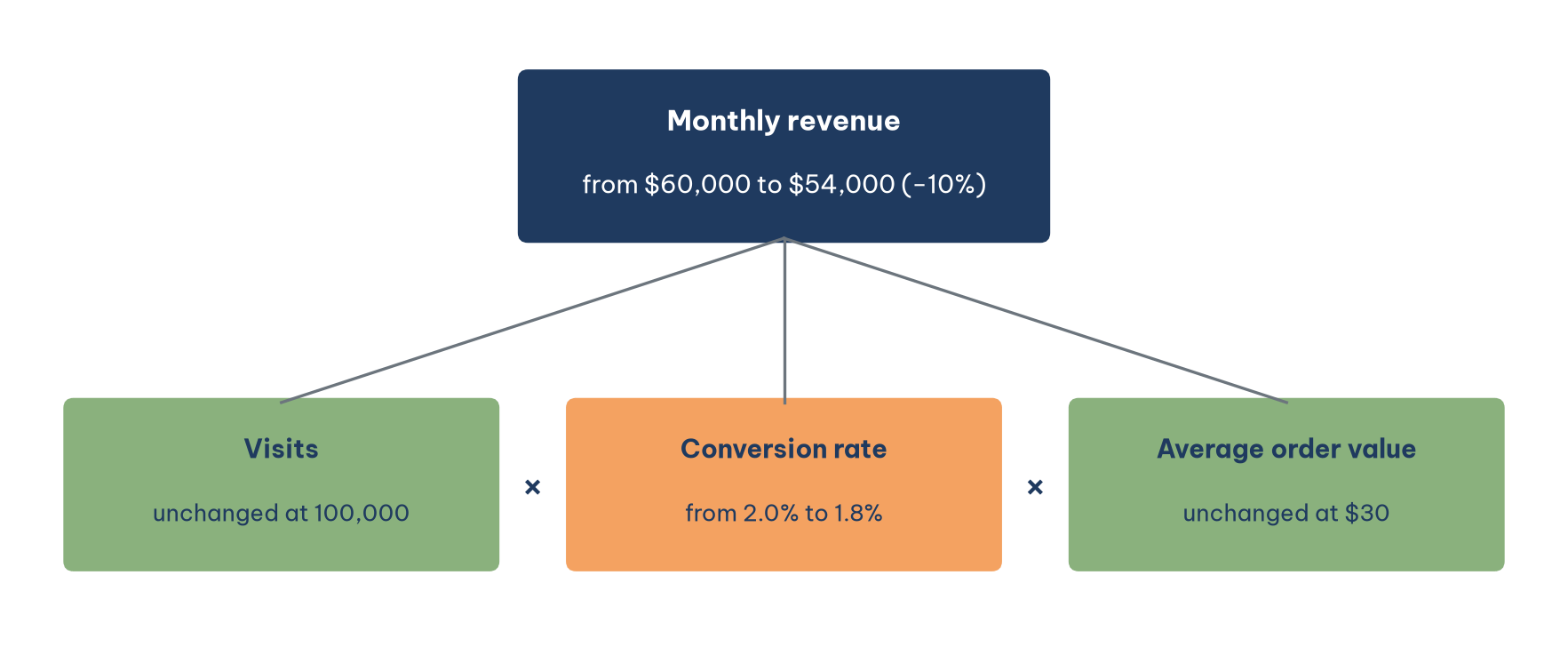
Figure 1 immediately answers the question the five-hypothesis meeting could not. Visits held at 100,000 and the average order value stayed at $30, so the entire $6,000 fall sits in the conversion rate, which slipped from 2.0% to 1.8%. Three of the five hypotheses can be dropped at once: a search algorithm change and failing advertising would have reduced visits, while a competitor's price cut would usually pull down either visits or order value, yet neither component changed. The same approach is known in finance as DuPont analysis, which splits return on equity into profit margin, asset turnover and financial leverage, and in management accounting as price and volume variance analysis (Richardson & Watson, 2024).
When more than one component moves at once, a multiplicative identity has a convenient property: the natural logarithm of a product is the sum of the logarithms of its parts. The log change of revenue therefore splits exactly into the log changes of visits, conversion rate and order value, and each term's share of the total tells you how much of the change that component accounts for. In this store, the log change of revenue is ln(0.9) ≈ −0.105, and all of it comes from the conversion rate term.
2.2. Decomposing by process steps
Once we know the conversion rate fell, the next question is at which stage of the purchase journey. Funnel analysis splits the journey into steps and measures the share of customers who move on at each step. Table 3 gives the store's counts for the two months, and Figure 2 sets the step-by-step rates side by side.
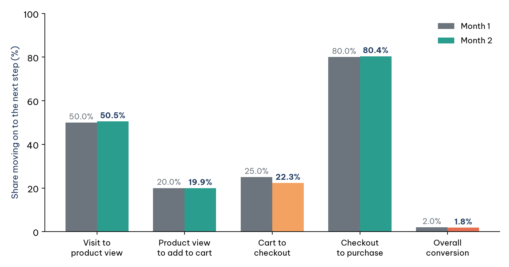
In Figure 2, the overall conversion rate falls by a tenth, from 2.0% to 1.8%. Placing the two funnels side by side, three steps are virtually unchanged; the decline is concentrated in the step from cart to checkout, where the share moving on falls from 25.0% to 22.3%. The log decomposition from Section 2.1 makes this precise: the cart-to-checkout step accounts for about 109% of the fall in conversion, while the other three steps taken together offset the extra 9%. The decomposition has located the change, but it has not said why. A payment gateway error, a new shipping fee or a redesign of the cart page are all hypotheses still to be tested. The funnel was born in marketing, but decomposing by steps works for any multi-stage process, from loan applications moving through credit review to candidates moving through rounds of hiring.
The other two axes complement this work. Drill-down summarizes data at increasingly detailed levels, like peeling the layers of an onion: viewed by day, the checkout rate might drop on one particular date that coincides with a website update (Sharda et al., 2024). Cohort analysis splits customers by the period in which they joined, which separates a change in how existing customers behave from a change in the kind of customers arriving. One trap of decomposing by data dimensions deserves a warning. When the mix of groups changes, the aggregate can move in the opposite direction from every one of its groups, a pattern known as Simpson's paradox, so a decomposition by segment should always show the size of each segment alongside its rate.
3. Reason about the root cause
This section turns the location found by decomposition into a chain of reasoning about why the change happened.
Decomposition says where the change is; qualitative techniques help reason about why. Root cause analysis is the process of identifying the factors that produced a change, and there may be more than one root cause. During the analysis it helps to distinguish four kinds of factors: the true root cause; unrelated factors; correlated factors, which are merely other symptoms of the same cause; and contributing factors in the chain of events. A useful habit is to place the suspected factors on a timeline, remembering that a cause may occur weeks before the change becomes visible.
The simplest tool is the 5 Whys, which originated in the Toyota Production System: ask "why" about five times to move from symptom to root. Applied to the store: revenue fell because the conversion rate fell; the conversion rate fell because more customers abandoned at the cart step; they abandoned at the cart because the shipping fee now appears for the first time at that step; the fee appears late because the new design removed the shipping estimate from the product page; the estimate was removed because the release process for design changes has no step that checks the effect on conversion. The root cause is not "the conversion rate fell" but the missing check in the release process.
The 5 Whys is cheap and fast, but it depends on the knowledge of the person asking and easily misses branches when a problem has several. For those cases there is the fishbone diagram (also called the Ishikawa diagram): the problem sits at the head of the fish, and groups of causes such as product, price, channel, promotion and process radiate out like bones, each group splitting into sub-causes. The fishbone diagram bridges qualitative reasoning and quantitative checking: from each branch the analyst chooses where to drill into the data. For problems that keep coming back after they are fixed, or get worse precisely because they were fixed, the arrow of causation no longer runs in one direction, and systems thinking with its feedback loops is the better tool.
4. Three levels of conclusion
This section separates three kinds of diagnostic conclusion and shows how to word each one so that it claims no more than the evidence supports.
A diagnostic report can offer three kinds of conclusion that differ greatly in strength, and the most common mistake is presenting a weak kind as if it were a strong one. Table 4 sets out the three levels.
The decomposition in Section 2 delivers a level-two conclusion: it shows where the change is, not why. The 5 Whys chain in Section 3 offers a plausible causal hypothesis, but it is not yet evidence. To reach level three, the store needs an experiment: show the shipping estimate again to a randomly selected half of visitors and compare the checkout rates of the two groups, which is a standard A/B test. Jumping straight from correlation to causation is unsafe because a third factor, such as a seasonal change in the kind of customer, can move both quantities at once.
A credible diagnostic conclusion must also stand up to alternative explanations. An effective method is to write down, before looking at the numbers, the trace each hypothesis would leave in the data: in which group, at what time, in which metric. The "slow season" hypothesis would reduce visits. The "competitor price cut" hypothesis would reduce visits and lower the conversion rate at every step. The "cart page design" hypothesis would hurt only one step. The data in Figure 2 match only the third.
AI tools help with listing hypotheses and building a fishbone diagram, because they generate branches faster than a meeting does. But AI also tends to conclude beyond the evidence, writing "the cause is…" when the data show only an association. Before sending a report, reread every concluding sentence, whether a person or a machine wrote it, and ask: what level does the evidence reach, and does the wording claim more than that level?
Conclusion
Finding the cause of a falling metric is an ordered process. Set an expectation first, so that you know what counts as an anomaly. Decompose to locate the change: by identity, the store's $6,000 drop in revenue sits entirely in the conversion rate; by funnel, it sits in the step from cart to checkout. Only then reason about the root cause with the 5 Whys or a fishbone diagram, checking each hypothesis against the trace it would leave in the data.
Conclusions must be worded to match the evidence: association, contribution or causation. Decomposition tells you where, not why; only a controlled experiment allows you to say "this change caused that result". The five-hypothesis meeting at the start of this article needed only a decomposition table to rule out four hypotheses and one experiment to confirm the one that remained.
References
Richardson, V. J., & Watson, M. W. (2024). Introduction to business analytics. McGraw Hill. https://www.mheducation.com/highered/product/introduction-business-analytics-richardson-watson/9781265450175.html
Sharda, R., Delen, D., & Turban, E. (2024). Business intelligence, analytics, data science, and AI: A managerial perspective (5th ed.). Pearson. https://www.pearson.com/en-us/subject-catalog/p/business-intelligence-analytics-data-science-and-ai/P200000009781
Discussion about this post