Decision Trees for Decisions Under Risk: Expected Value, Sensitivity and the Value of Information
How payoff tables, decision trees, risk profiles, Bayes’ theorem and utility turn a boardroom argument into a clear, defensible strategy


Key takeaways
Without probabilities, the maximax, maximin and minimax regret criteria give three different answers to the same payoff table, because they encode three different attitudes toward risk.
A decision tree with probabilities lets you compute expected values by rolling back from right to left; in the worked example the large project wins with an expected value of $14.2 million.
The highest expected value can hide a 20% chance of a $9 million loss, and the choice flips if the probability of strong demand falls below 0.70, only 0.1 away from the estimate.
Perfect information is worth at most $3.2 million; a real market study with a known track record is worth about $1.62 million, and the output is a strategy, not a single choice.
When a bad outcome is hard to absorb, an exponential utility function shows how a firm's risk tolerance can reverse the expected value ranking.
Every organization eventually faces a decision that is large, made once and shaped by things nobody can know in advance. A manufacturer decides how big a new plant should be before it knows next year's demand. A pharmaceutical company decides whether to fund a costly late-stage trial. A retailer decides how much seasonal stock to order months before the season starts. In each case the meeting tends to split into camps: the optimists who want to go big, the cautious who want to stay small and a third group who want more data before anyone commits. All of them have a point and none of them can prove it by argument alone.
Decision analysis is the toolkit for exactly this situation. It applies when there are a few discrete alternatives (not the endless continuum of an optimization problem) and the result of each depends on uncertain events outside the decision maker's control. Because the alternatives can be listed, each can be evaluated and compared openly. This article walks through the whole toolkit using one classic case that runs through Camm et al. (2024): Pittsburgh Development Corporation (PDC), a real estate developer choosing the size of a condominium project. If demand is strong, the largest project earns $20 million; if demand is weak, it loses $9 million. The smallest project is far safer but can earn at most $8 million. The board has the same three camps described above. All amounts in the case are in U.S. dollars.
Section 1 sets up the payoff table and three criteria that need no probabilities. Section 2 introduces decision trees and expected value. Section 3 looks at risk profiles and at how sensitive the decision is to the probability estimate. Section 4 puts a number on the value of information, perfect and imperfect, using Bayes' theorem. Section 5 brings in attitudes toward risk through utility functions. Section 6 summarizes which tool fits which situation and where AI helps and where it does not.
1. The payoff table and three criteria without probabilities
This section organizes the problem in a payoff table and shows why three common criteria disagree.
A payoff table lays out the problem systematically. Rows are the alternatives the decision maker can choose; columns are the states of nature, the scenarios outside the decision maker's control; each cell is the resulting payoff. PDC has three alternatives (a small project of 30 units, a medium project of 60 units and a large project of 90 units) and two states of nature (strong demand and weak demand). Table 1 shows the payoffs together with three summary columns used below.
When no probabilities are available for the states of nature, three widely taught criteria give three different answers. The maximax criterion picks the alternative with the best payoff in its best case: the large project, because $20 million is the highest number in the table. The maximin criterion picks the alternative with the best payoff in its worst case: the small project, which guarantees at least $7 million. The minimax regret criterion first computes the regret of each cell, the gap between that payoff and the best payoff in the same column, and then picks the alternative whose largest regret is smallest. If demand is strong, the small project falls $12 million short of the large one; if demand is weak, the large project falls $16 million short of the small one. The medium project never misses the best result by more than $6 million (14 versus 20 under strong demand, 5 versus 7 under weak demand), so minimax regret chooses the medium project.
Three answers are not a failure of the method. They reflect three philosophies about risk, and they map neatly onto the three camps on the board: the optimist reasons by maximax, the cautious member by maximin and the member who fears looking foolish afterward by minimax regret. The weakness all three share is that they ignore how likely each state is. A project that loses money only in a very unlikely scenario is treated the same as one that loses money in a likely scenario. As soon as the probabilities can be estimated, even subjectively by experienced people, a stronger criterion becomes available.
2. Decision trees and expected value
This section shows how a decision tree represents the problem and how expected value ranks the alternatives.
A decision tree is a diagram of a sequence of decisions and uncertain outcomes. Squares are decision nodes, where the decision maker chooses a branch. Circles are chance nodes, where one of several uncertain outcomes occurs with a stated probability. Branches leaving the same node are mutually exclusive, and the probabilities on the branches leaving a chance node sum to one. The term should not be confused with the decision tree in machine learning, a classification algorithm that learns splitting rules from data. The two share a name and a branching shape but serve different purposes: one structures a choice, the other predicts a label.
The expected value (EV) of an alternative is the probability-weighted average of its payoffs: multiply each payoff by the probability of its state and add the products. Suppose the board estimates the probability of strong demand at 0.8 and of weak demand at 0.2. Figure 1 draws the tree with these probabilities and the expected value of each alternative.
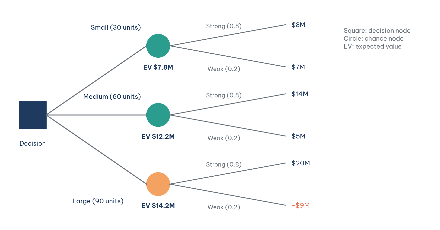
From Figure 1, the expected value of the small project is 0.8 × 8 + 0.2 × 7 = $7.8 million, of the medium project 0.8 × 14 + 0.2 × 5 = $12.2 million and of the large project 0.8 × 20 + 0.2 × (−9) = $14.2 million. The expected value criterion chooses the large project.
A decision tree is solved by rolling back from right to left. At each chance node, compute the expected value of the branches that leave it; at each decision node, keep the branch with the highest value and prune the rest. In a one-stage tree like Figure 1 this looks trivial, but the same procedure handles trees with several stages of decisions and uncertain events, such as the "research first, then decide" tree in Section 4. The power of the method lies less in the arithmetic than in the discipline it imposes: every alternative, every uncertain event and every probability must be written down where others can see and challenge it.
3. Risk profiles and sensitivity to probabilities
This section looks behind the single expected value number, first at the spread of outcomes and then at how much the choice depends on the probability estimate.
The figure of $14.2 million conceals something that a risk profile reveals. A risk profile is the probability distribution of the payoffs of one alternative, and Table 2 lists them for the three projects.
The large project carries a 20% chance of losing $9 million, while the medium project never loses money. A risk-averse decision maker may reasonably choose the medium project and give up $2 million of expected value (14.2 minus 12.2) in exchange for that safety. Expected value is not wrong, but it is not the only legitimate criterion, and Section 5 shows how to make the trade-off explicit.
There is a second reason for caution. Subjective probabilities tend to be optimistic, so the next step is to ask how sensitive the decision is to them. Let p be the probability of strong demand. The expected values of the three alternatives are then three straight lines in p: 7 + p for the small project, 5 + 9p for the medium project and −9 + 29p for the large project. Figure 2 plots them.
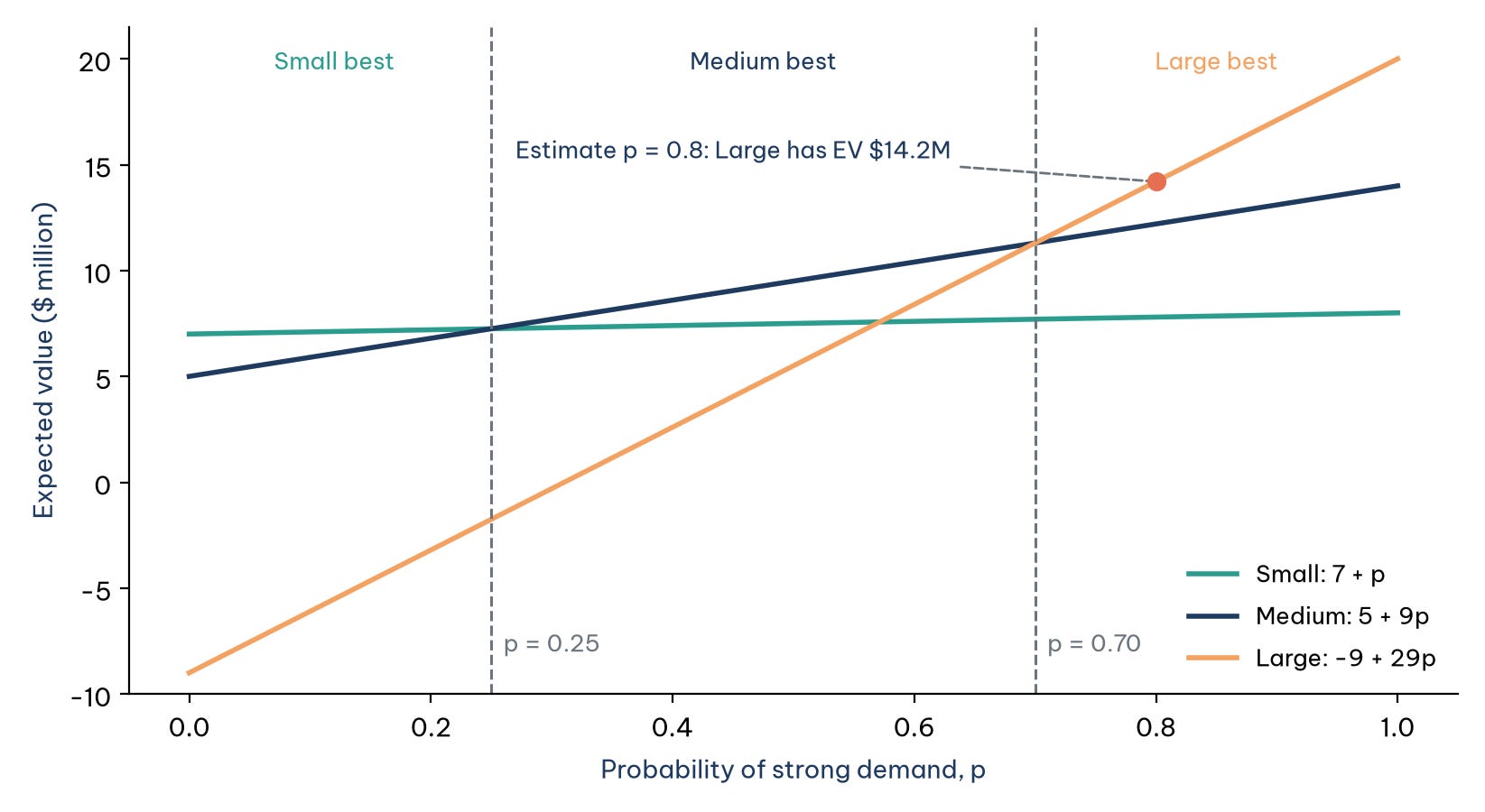
The breakpoints come from setting the lines equal. The small and medium projects tie when 7 + p = 5 + 9p, that is at p = 0.25, where both are worth $7.25 million. The medium and large projects tie when 5 + 9p = −9 + 29p, that is at p = 0.70, where both are worth $11.3 million. Figure 2 shows that the large project is best only when the probability of strong demand exceeds 0.70, the small project is best below 0.25 and the medium project is best in between. The board's estimate of 0.8 sits just 0.1 above the upper threshold. If the board is even slightly overconfident, the recommended decision changes.
Camm et al. (2024) offer a practical rule: if a small change in an input changes the recommended alternative, that input is sensitive and deserves more careful estimation. Here the probability of strong demand is clearly sensitive, while the payoffs of the small project hardly matter. The same logic underlies what-if analysis in spreadsheets: rather than trusting a single point estimate, find the range over which the conclusion holds and ask whether reality could plausibly fall outside it.
4. The value of information
If the probability is that sensitive, how much is it worth paying to learn more? The third camp on the board was asking exactly this question, and decision analysis gives it a numerical answer.
4.1. Perfect information
Imagine an oracle who could tell PDC in advance which state of nature will occur. If demand will be strong, the company builds the large project and earns $20 million; if demand will be weak, it builds the small project and earns $7 million. Before the oracle speaks, strong demand is still expected with probability 0.8, so the expected value with perfect information is 0.8 × 20 + 0.2 × 7 = $17.4 million, compared with $14.2 million without it. The difference of $3.2 million is the expected value of perfect information (EVPI).
EVPI is a ceiling on what any study is worth, because no real study is perfect. Its practical use is as a quick filter: a market research proposal priced at $4 million can be rejected at once, without further calculation.
4.2. Imperfect information and Bayes' theorem
Real research is imperfect, and Bayes' theorem tells us how much it is worth. Suppose a market research firm has a track record: when demand really was strong, it reported a favorable outlook 90% of the time; when demand was weak, it still reported a favorable outlook 25% of the time. Combining this track record with the prior probabilities gives the quantities in Table 3.
A favorable report raises the probability of strong demand from 0.8 to 0.935; an unfavorable report cuts it to 0.348, well inside the zone where Figure 2 says the medium project is best. With these updated (posterior) probabilities, the tree now has two stages: first the research result, then the size decision. Figure 3 shows it rolled back.
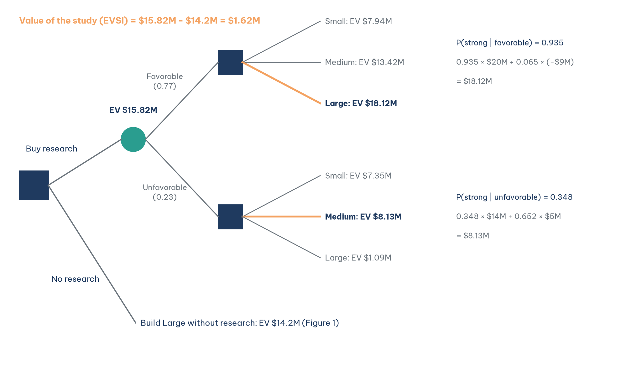
After a favorable report, the large project has an expected value of 0.935 × 20 + 0.065 × (−9) ≈ $18.12 million, ahead of the medium project at $13.42 million. After an unfavorable report, the medium project is best at 0.348 × 14 + 0.652 × 5 ≈ $8.13 million, while the large project drops to about $1.09 million. The expected value of the whole strategy "buy the research, then decide" is 0.77 × 18.12 + 0.23 × 8.13 ≈ $15.82 million. Subtracting the $14.2 million available without research gives the expected value of sample information (EVSI) of about $1.62 million. PDC should buy the study if it costs less than that. The ratio of EVSI to EVPI, 1.62 / 3.2 ≈ 0.51, is the efficiency of the study: this research captures about half the value of perfect information.
A note on precision. Hand calculations often round the posterior probabilities to two decimals (0.94 and 0.35). Carried through the tree, that rounding gives an expected value of about $15.93 million and an EVSI of about $1.73 million, about $115,000 more than the exact figure. The difference does not change the decision in this case, but it could when a quoted price falls between the two numbers, which is a good reason to let a spreadsheet carry full precision.
The output of this analysis is not a single decision but a strategy: a rule saying what to do for each possible result that is not yet known. "Buy the research; if the report is favorable, build large; if it is unfavorable, build medium" is a complete answer to the board's question, and each of the three camps can see its own concern reflected in it.
The trap in this section is misreading the value of a signal. Posterior probabilities often surprise people, experts included. A classic medical example makes the point: a disease affects 1% of the population, and a test gives 10% false positives and 5% false negatives. A person who tests positive has only about an 8.8% chance of having the disease. Out of 10,000 people, 100 have the disease and 95 of them test positive, but 990 of the 9,900 healthy people also test positive, so only 95 of the 1,085 positives are true (Albright & Winston, 2025). A "favorable" market report or a "positive" fraud alert must be read the same way: what a signal is worth depends both on its accuracy and on the prior probability of the event it signals.
5. Attitudes toward risk
This section explains when expected value is the right yardstick and how utility functions handle the cases where it is not.
Using expected value implicitly assumes that the decision maker is risk neutral. That assumption is reasonable when the amounts are small relative to the decision maker's wealth and the decision is repeated many times, such as a retail chain choosing a weekly promotion: over many repetitions, good and bad draws average out. It is not reasonable for a large decision made once. An extreme example makes this vivid. A bet that wins $1,000 with probability 0.9999 but loses $500,000 with probability 0.0001 has a positive expected value of about $950 (0.9999 × 1,000 − 0.0001 × 500,000), yet it would be a disaster for anyone who is not very wealthy (Sharda et al., 2024).
The tool for building risk attitude into the calculation is a utility function. Instead of averaging money, we average the "utility" of money, which grows more and more slowly as money increases and falls steeply for losses. A common form is the exponential utility function, U(x) = 1 − e^(−x/R), with a single parameter R called the risk tolerance. Albright and Winston (2025) give a practical way to estimate it: R is roughly the largest amount for which the decision maker would accept a 50-50 gamble between winning R and losing R/2. A smaller R means more risk aversion.
The result of a utility calculation is easiest to read as a certainty equivalent (CE): the sure amount that the decision maker would consider just as good as the risky alternative. For the exponential function, CE = −R × ln(E[e^(−X/R)]), where X is the uncertain payoff. Table 4 applies this to the PDC projects at p = 0.8 for several levels of risk tolerance.
The ranking changes with risk tolerance. A firm with R of $10 million or $20 million, for which a $9 million loss would be painful, should prefer the medium project; its certainty equivalent for the large project is far below the $14.2 million expected value. The two projects tie at a risk tolerance of about $35.6 million, and only above that does the large project win. As R grows, every certainty equivalent approaches its expected value, which is why expected value is the special case of a decision maker with unlimited risk tolerance. For the same project, a firm with a small R may rationally say no while a firm with a large R says yes (Albright & Winston, 2025). Utility does not replace expected value; it tells you how far expected value can be trusted by the people who would have to absorb the bad outcome.
6. Choosing the tool and the role of AI
This section pulls the toolkit together and marks the boundary between what software can do and what people must own.
Table 5 summarizes which tool fits which decision situation.
An AI assistant can build a decision tree from a verbal description and compute every number in this article, including the Bayesian step that is easy to get wrong by hand, and it can rerun the sensitivity analysis or the utility table in seconds. But the two most important inputs must come from people who are accountable for them: the subjective probabilities of the states of nature and the attitude toward risk. A decision tree built by AI with probabilities "guessed" by AI is a precise calculation resting on an assumption that nobody owns. The useful division of labor is the opposite: people supply and defend the probabilities, the payoffs and the risk tolerance, and the software does the arithmetic and shows how the answer moves when those inputs move.
Decision analysis also sits in a particular place among types of analytics. Descriptive and predictive analytics tell a manager what has happened and what is likely to happen; decision analysis belongs to prescriptive analytics, because it ends with a recommended course of action and an explicit account of the assumptions behind it (Camm et al., 2024).
Conclusion
The three camps on the board at the start of this article were really using three different criteria: maximax, maximin and an intuition about the value of information. Decision analysis does not choose for them, but it shows which assumptions each choice rests on. With a probability of 0.8 for strong demand, the large project has the highest expected value at $14.2 million. Yet it carries a 20% chance of a $9 million loss, and the decision reverses if the probability falls below 0.70.
The value of information can be measured. Perfect information is worth at most $3.2 million, and a real market study with a 90% hit rate and a 25% false alarm rate is worth about $1.62 million. What the study buys is a strategy: build large after a favorable report, build medium after an unfavorable one. When bad outcomes are hard to absorb, risk profiles and utility functions are a reminder that the highest expected value is not automatically the right choice: a developer with a risk tolerance below about $35.6 million should prefer the medium project even before any research is done.
References
Albright, S. C., & Winston, W. L. (2025). Business analytics: Data analysis and decision making (8th ed.). Cengage Learning. https://www.cengage.ca/c/new-edition/9780357984581/
Camm, J. D., Cochran, J. J., Fry, M. J., & Ohlmann, J. W. (2024). Business analytics (5th ed.). Cengage Learning. https://www.cengage.com/c/business-analytics-5e-camm-cochran-fry-ohlmann/9780357902202/
Sharda, R., Delen, D., & Turban, E. (2024). Business intelligence, analytics, data science, and AI: A managerial perspective (5th ed.). Pearson. https://www.pearson.com/en-us/subject-catalog/p/business-intelligence-analytics-data-science-and-ai/P200000009781
Discussion about this post