Benford's Law: Detecting Suspicious Numbers
The hidden order in first digits, how auditors use it to screen accounting data, and the limits you must respect before drawing conclusions


Key takeaways
In many real datasets the first digit is 1 about 30% of the time and 9 less than 5% of the time, following P(d) = log10(1 + 1/d).
The pattern follows from multiplicative growth and scale invariance, so it holds for data that are natural and span several orders of magnitude.
People who fabricate numbers tend to spread digits evenly, which makes Benford a useful screening tool in auditing, macroeconomic data, digital forensics and science.
A single summary statistic such as MAD can miss local fraud; first-two-digit tests reveal spikes just below approval thresholds.
A deviation is a red flag, not a verdict. Check whether the data should follow Benford at all, and confirm with documents.
We work with a great many numbers: financial statements, population data, scientific measurements. Faced with this sea of figures, human intuition tends to assume something very natural: randomness means even spread.
If you closed your eyes and picked any number from a newspaper or a report, you would expect the chance of it starting with 1, 2, 3 ... up to 9 to be the same, about 11.1%. But that intuition is wrong. In very many real datasets, the digit 1 comes first about 30% of the time, while 9 comes first less than 5% of the time.
This phenomenon is called Benford's law, or the first-digit law. It is not magic but a consequence of how numbers grow in the real world. And because people are very good at making up stories but very bad at making up numbers that "look random", the law has become a familiar screening tool for auditors and data analysts. As this article shows, however, it also has important limits that users must understand to avoid wrongful conclusions.
The article has seven parts. Section 1 recounts how the law was discovered and states it. Section 2 explains why the digit 1 dominates. Section 3 reviews fields of application, from auditing to digital forensics. Section 4 shows how to run the test yourself in Excel and Python. Section 5 works through an expense-audit example with simulated data, showing how the law is used in practice and why looking only at the first digit is not enough. Section 6 discusses when the law does not apply and how to interpret results cautiously. Section 7 places Benford within the wider toolkit of diagnostic analytics.
1. What is Benford's law?
The story begins in 1881, not with Frank Benford but with the American astronomer Simon Newcomb. Working in a library, Newcomb noticed something odd: books of logarithm tables, a common calculating tool at the time, were most worn on the first pages, which held numbers starting with 1 and 2. The last pages, with numbers starting with 8 and 9, were still almost new (Newcomb, 1881).
Newcomb published the observation in a short note, but it was soon forgotten. Only in 1938 did Frank Benford, a physicist at General Electric, rediscover the phenomenon independently. Going beyond observation, Benford checked more than 20,000 numbers from 20 different datasets: river drainage areas, atomic weights, populations, even numbers appearing in Reader's Digest (Benford, 1938). The datasets, utterly different in nature, all came close to the same distribution. The law is named after him in recognition of his systematic work.
Benford's law describes how often each first digit appears in many real datasets. The probability P that a digit d (from 1 to 9) appears first is:
P(d) = log10(1 + 1/d)
(where log10 is the base-10 logarithm)
Applying the formula gives the distribution in Table 1 and Figure 1.
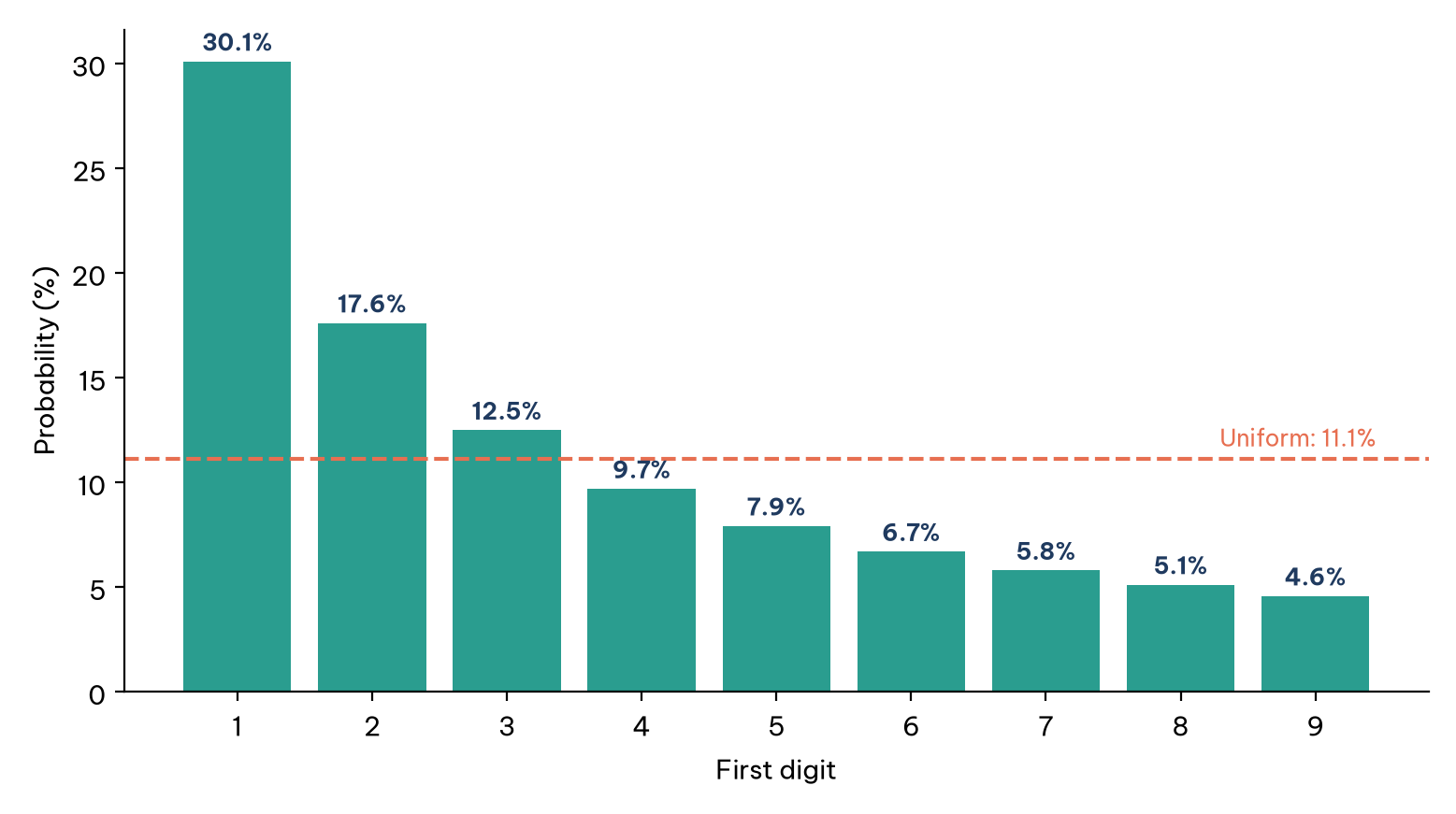
The digit 1 appears about 6.5 times as often as 9. If a set of accounting data is prepared honestly and is of a suitable type, it will usually come close to this curve. Conversely, when people deliberately invent or falsify figures, they tend to fall into a psychological trap: spreading the numbers evenly because they think that is what "random" looks like. The very effort to make the data look fair becomes the giveaway. But why does the real world "favour" the digit 1? That is the question of the next section.
2. Why does the digit 1 dominate?
There are two complementary explanations: an intuitive one based on growth, and a mathematical one based on invariance.
2.1. Growth and the logarithmic scale
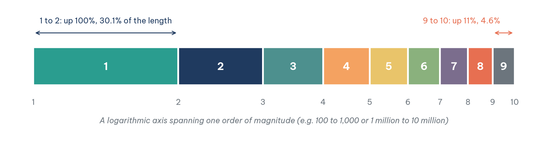
The easiest explanation uses a savings account. Imagine an account with a balance of USD 100. To reach USD 200, moving from a first digit of 1 to 2, it has to grow by 100%. Doubling takes a long time, so the balance "stays" in the 1-range for a long while. But once the account reaches USD 900, getting to USD 1,000, from 9 back to 1, takes only about 11% growth. Because growing 100% takes much longer than growing 11%, you are far more likely to catch a number in its "1 phase" than in its "9 phase".
Figure 2 shows the same idea on a logarithmic axis. On this axis, distance corresponds to growth rate rather than difference. The segment from 1 to 2 takes up 30.1% of an order of magnitude, while the segment from 9 to 10 takes up only 4.6%. If values are spread evenly on a log scale, as is typical of data growing exponentially, the first-digit shares are exactly these segment lengths.
2.2. Scale invariance
The second explanation is mathematical: scale invariance. If there were a general law of first digits for prices in one currency, it would have to hold when converted to dollars or euros, that is, when every value is multiplied by a constant. Hill (1995) proved that the only distribution with this property is Benford's, and also showed that mixing many different distributions tends to converge on Benford. Data generated by many multiplications, by growth, or by combining many sources on different scales therefore tend to come close to Benford.
Both explanations also tell us when not to expect Benford: when data do not span several orders of magnitude, or are constrained by human-imposed limits. Section 6 returns to this. First, let us see where the law is used.
3. Practical applications of Benford's law
Benford's law is not just a statistical theory on paper. It has become a tool of forensic accounting and data quality assurance. Table 2 summarizes five main groups of applications and how reliable each is; the subsections below go into detail.
3.1. Detecting financial fraud
This is the classic application. When people try to "cook the books" or embezzle funds, they often try to spread the numbers evenly. Fraudsters think that for data to look random, every digit must appear equally often, whereas natural randomness favours small digits.
Auditors scan the dataset (invoices, cheques, ledger entries). If the distribution shows unusual spikes at large digits such as 7, 8 and 9, or just below approval thresholds (for example USD 4,900 to avoid a USD 5,000 approval level), that is a signal to look more closely.
The Wayne J. Nelson case of 1993 is the classic example. Nelson, a manager in the Arizona State Treasurer's office, embezzled nearly USD 2 million through 23 cheques paid to a fictitious vendor. He kept each cheque below USD 100,000 to avoid an extra approval threshold and tried not to repeat amounts. As a result, most of the amounts began with 7, 8 or 9, the opposite of Benford. Mark Nigrini uses the case as an example in his work on forensic accounting (Nigrini, 2012).
Be cautious with widely circulated examples, too. Many popular articles claim that Enron's figures deviated from Benford when reanalysed. This claim is often repeated but rarely backed by published research; moreover, Enron's fraud lay mainly in accounting treatment (special-purpose entities, revenue recognition), which first-digit tests are poorly placed to detect.
3.2. Checking macroeconomic statistics
At the national level, economic data can face political pressure: governments may want to flatter figures on budget deficits, public debt or inflation. Rauch et al. (2011) applied Benford to the macroeconomic data that EU countries reported to Eurostat in 1999–2009. Greece's data showed the largest deviation, consistent with Greece later admitting to misreporting its budget deficit. This result is a warning signal consistent with known facts, not independent proof.
3.3. Screening election data: a controversial application
Vote counts at polling stations can span several orders of magnitude, so there have been attempts to use Benford to screen for anomalies. But this is the most controversial application. After Iran's 2009 presidential election, some researchers analysed the digits of vote counts and argued there were signs of irregularity; but the most prominent analysis (Beber & Scacco, 2009) did not use Benford but the last digits, which should be uniformly distributed if the figures are untouched. Deckert et al. (2011) warn that vote counts usually do not naturally follow Benford, because polling districts are often designed to be of similar size, so Benford tests on election data easily give wrong results in both directions.
3.4. Digital forensics and social networks
In the digital world, Benford has new applications. For digital images, it is not pixel intensities themselves but the discrete cosine transform (DCT) coefficients used in JPEG compression that follow a generalized form of Benford's law (Fu et al., 2007). Images compressed several times or spliced together can distort this distribution. It is one of many image-forensics techniques, not enough on its own to detect modern fakes. For social networks, Golbeck (2015) showed that the numbers of friends and followers of accounts in many networks come close to Benford, while fake accounts (bots) may have connection counts following artificial patterns that distort the distribution.
3.5. Validating scientific data
Many kinds of scientific measurement span several orders of magnitude and come close to Benford. If figures are altered to achieve a desired result, the distribution may break. Some researchers and reviewers have used Benford to scan datasets submitted with papers quickly, as a screening step to catch academic fraud or faulty instruments early. As in other fields, though, you must first check whether the specific type of data should follow Benford.
Across these five groups, the common thread is that Benford is most useful when the data are monetary amounts or natural measurements that are widely spread, and when the results are used to narrow down rather than to conclude. The next section shows how to run the test yourself.
4. Testing for Benford in Excel and Python
The basic test has three steps: take the first digit of each value, calculate the share of each digit from 1 to 9, and compare with the theoretical shares.
In Excel or Google Sheets. Suppose column A contains (positive) amounts. In column B, extract the first digit with =VALUE(LEFT(TEXT(A2,"0"),1)) (use semicolons instead of commas depending on your regional settings). Use COUNTIF to count the rows whose first digit is 1, 2, …, 9, divide by the total number of rows, and plot a bar chart next to the theoretical line =LOG10(1+1/d).
In Python. The code below compares two simulated sets of 5,000 invoices: a "natural" set spanning several orders of magnitude, and a "fabricated" set spread evenly between 1 and 10 million.
import numpy as np

def first_digit(x):
    x = np.abs(x[x != 0])
    return (x / 10 ** np.floor(np.log10(x))).astype(int)

def benford_test(amounts, label):
    d = first_digit(np.asarray(amounts, dtype=float))
    observed = np.array([(d == k).mean() for k in range(1, 10)])
    expected = np.log10(1 + 1 / np.arange(1, 10))
    mad = np.abs(observed - expected).mean()  # mean absolute deviation
    print(f"{label}: share of 1 = {observed[0]:.1%}, share of 9 = {observed[8]:.1%}, MAD = {mad:.4f}")

rng = np.random.default_rng(7)
natural = rng.lognormal(mean=13, sigma=1.5, size=5000)          # 5,000 invoices spanning several orders of magnitude
fabricated = rng.uniform(1_000_000, 9_999_999, size=5000)       # "made up", spread evenly from 1 to 10 million
benford_test(natural, "Natural invoices")
benford_test(fabricated, "Fabricated uniform invoices")
Output:
Natural invoices: share of 1 = 30.0%, share of 9 = 5.0%, MAD = 0.0031
Fabricated uniform invoices: share of 1 = 11.2%, share of 9 = 12.0%, MAD = 0.0609
Figure 3 visualizes the result: the natural invoices track the Benford line closely, while the fabricated ones are almost flat.
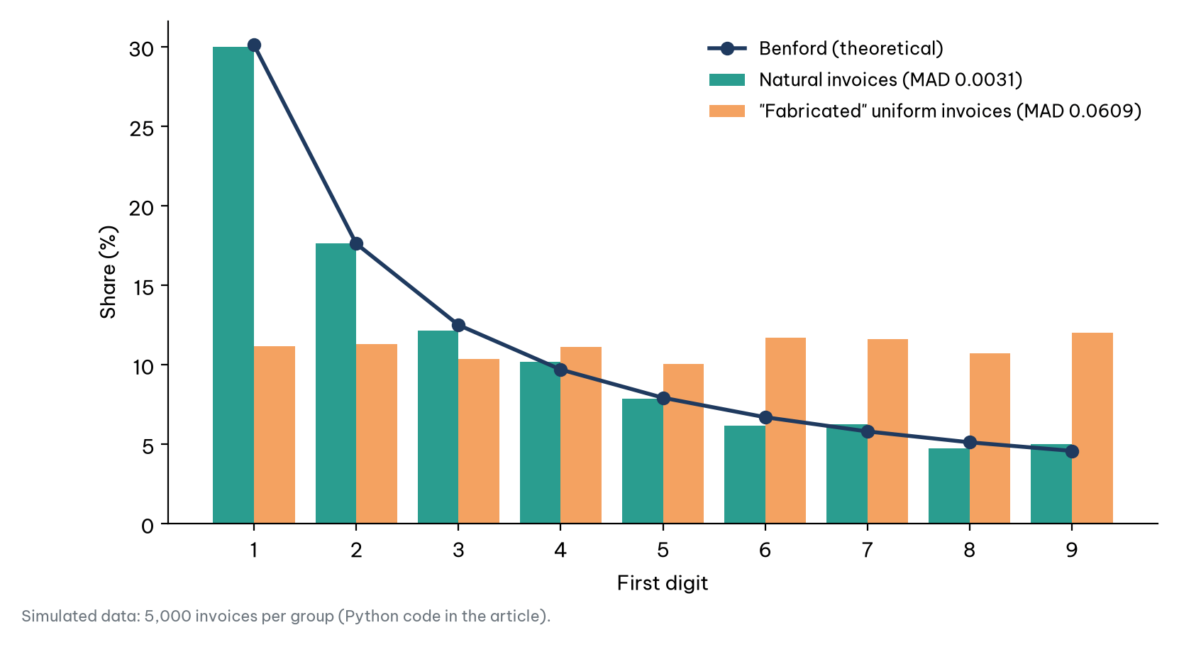
MAD (mean absolute deviation) is the average absolute difference between the observed shares and the Benford shares. Unlike the chi-squared test, which almost always "rejects" with very large datasets, MAD depends little on sample size, so auditors favour it for large datasets. Nigrini (2012) proposes the reference thresholds in Table 3.
By these thresholds, the natural invoices (MAD 0.0031) conform closely and the fabricated ones (MAD 0.0609) do not. But real fraud is rarely as crude as "spread it evenly". The example in the next section shows a subtler situation, and why an overall MAD figure can miss it.
5. An expense-audit example: when the first digit alone is not enough
Consider a common internal-control situation. A company requires every expense invoice of USD 2,000 or more to be approved by the chief financial officer. Some employees, to avoid this step, split large expenses into several invoices, each between USD 1,800 and just under USD 2,000. This is not necessarily embezzlement, but it breaches procedure and may hide improper spending.
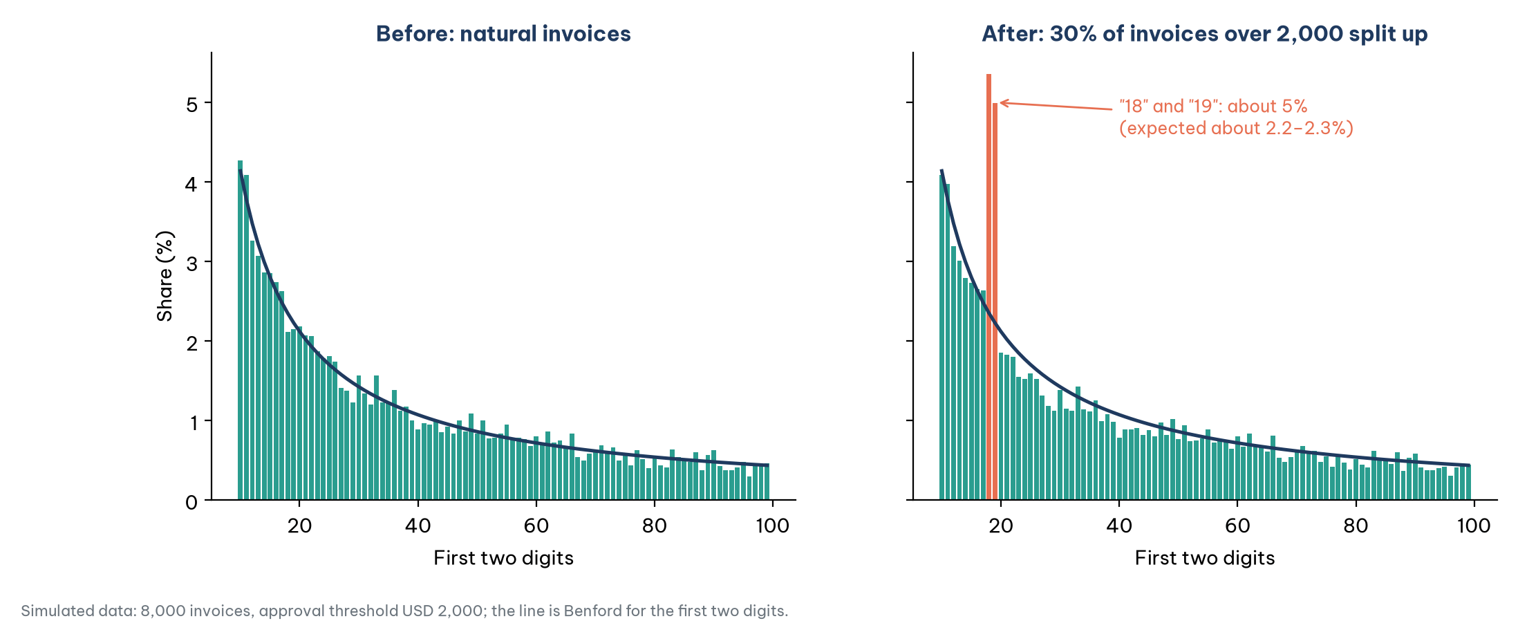
To see how far Benford can detect this, we simulated 8,000 "natural" invoices, of which 885 exceeded the USD 2,000 threshold. We then assumed that 30% of those (265 invoices) were split into 796 new invoices, most worth USD 1,800–1,999. The results are as follows.
With the first-digit test, the share of 1 rose from 30.0% to 35.4%, and MAD rose from 0.0019 to 0.0118. By Table 3, this is still "acceptable conformity". Looking only at the overall MAD, an auditor might conclude there was nothing to worry about.
With the first-two-digits test (10, 11, …, 99), the picture is much clearer (Figure 4). The shares of invoices starting with "18" and "19" rose to about 5%, more than double the expected 2.2–2.3%, forming two bars that stand out sharply. Notably, the two-digit MAD rose only from 0.0009 to 0.0017, still "acceptable", because the anomaly is concentrated in two of 90 groups. The lesson: MAD tells you the overall fit, while fraud usually leaves local traces. Auditors need to look at each bar that sticks out, especially just below known thresholds, not just at one summary number.
From here the next audit steps are clear: filter the invoices starting with 18 and 19 hundred dollars, group them by requester, vendor and date, look for clusters of consecutive invoices from the same vendor whose total exceeds the threshold, and check them against source documents. Benford cannot prove who broke the rules; it only shows where to start looking among 8,531 invoices. In practice, auditors usually combine first-digit and first-two-digit tests with other checks such as searching for duplicate amounts (Nigrini, 2012).
The example also shows the law's limit: if the data are unsuitable to begin with, every comparison is meaningless. That is the subject of the final section.
6. When does Benford's law not work?
Powerful as it is, Benford's law is not a master key. Understanding its limits is a precondition for avoiding wrongful conclusions. Three groups of conditions need checking.
6.1. The data must be "natural" and widely spread
Benford's law applies only to data that arise naturally and span several orders of magnitude, for example from 100 to 1,000,000. Table 4 lists common kinds of data that do not follow Benford.
6.2. The sample must be large enough
Benford's law is a law of large numbers. If you analyse only 20 invoices, it is perfectly normal for them not to have exactly 30.1% starting with 1. For a meaningful analysis, a dataset usually needs hundreds, preferably thousands, of observations; for the first-two-digits test, with 90 groups, the sample-size requirement is higher still.
6.3. Interpret with care: a red flag is not a verdict
A deviation from Benford's law is a "red flag" signalling an anomaly, but it is never proof of guilt. Deviations can have legitimate causes: rules requiring transactions above a certain amount to be reported create distortions at the cut-offs; mergers, process changes or flat-price promotions change the mix of amounts; and data-entry errors happen. Even in the Section 5 example, invoices of USD 1,800–1,999 could come from an entirely legitimate framework contract with a fixed unit price.
Benford's law should therefore be seen as an initial screening tool for narrowing down suspicions and telling auditors where to start looking, not as a final judgment. This matters all the more when data-analysis results feed into internal reviews or official inspections: any conclusion of wrongdoing must rest on documents and explanations, not on a chart.
7. Benford within the diagnostic analytics toolkit
Section 6 stresses that a Benford red flag is not a verdict. So what comes after the red flag? The answer lies in how diagnostic analytics, the type of analysis that asks "why", organises its techniques.
7.1. Four groups of diagnostic techniques
Diagnostic techniques can be arranged into four groups by their role in the search for causes, as Figure 5 shows. A typical process starts with detection (what is unusual?), uses qualitative techniques to list possible causes, then uses quantitative and decomposition techniques to test and locate the real cause.
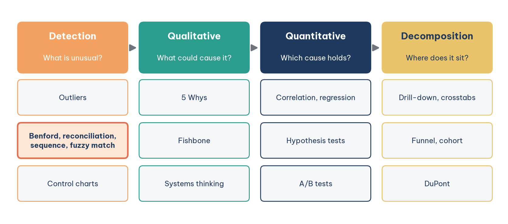
Figure 5 shows that Benford is only the opening move. Detection compares data with an expectation in order to pick out what needs explaining; for Benford, the expectation is the first-digit distribution of naturally occurring numbers. The comparison itself is descriptive; it becomes diagnostic only when it is connected to the steps that find and test causes.
7.2. Transaction tests that go with Benford
In accounting and auditing, Benford sits alongside other tests built on the same principle: compare the data with a constraint that correct data must satisfy (Nigrini, 2012; Richardson & Watson, 2024). Table 5 summarises five of them.
Apply Table 5 to the expense-audit example in Section 5. The first-two-digits test revealed an unusual spike in invoices just below the approval threshold. The next step is not to conclude fraud but to run the other tests on those same invoices: look for duplicates with the same supplier, date and similar amounts; fuzzy-match supplier names and addresses against the employee list; check the sequence of invoice numbers from each supplier. Only when signals overlap does the work move to the qualitative group, interviewing the people who raised and approved the invoices, and then to the quantitative group, comparing with other departments. One red flag is a question; several red flags on the same set of transactions are a lead.
Conclusion
Benford's law is a beautiful demonstration of mathematics' ability to find order among apparently chaotic numbers. From river drainage areas and city populations to the dry figures in an accounting ledger, the "dominance of the digit 1" appears wherever data grow naturally and span several orders of magnitude. The explanations from growth and from scale invariance show that this is not a coincidence but a necessary consequence.
In analytical work, the law's role is screening data integrity. For managers, auditors and data scientists, Benford is like a torch shone into dark corners, helping to narrow down suspicious points that the naked eye easily misses. But as the expense-audit example shows, the torch has to be pointed correctly: test the first two digits as well, watch for bars sticking out just below thresholds, and do not let one overall MAD figure lull you.
Next time you hold a financial report or a table of figures, glance down a column of numbers. If 1s are scarce and 9s unusually dense, ask two questions: does this kind of data follow Benford, and if so, what pushed it off course? That is where an investigation begins, not where it ends.
References
Beber, B., & Scacco, A. (2009, June 20). The devil is in the digits. The Washington Post. http://www.washingtonpost.com/wp-dyn/content/article/2009/06/20/AR2009062000004.html
Benford, F. (1938). The law of anomalous numbers. Proceedings of the American Philosophical Society, 78(4), 551–572. https://www.jstor.org/stable/984802
Deckert, J., Myagkov, M., & Ordeshook, P. C. (2011). Benford's law and the detection of election fraud. Political Analysis, 19(3), 245–268. https://doi.org/10.1093/pan/mpr014
Fu, D., Shi, Y. Q., & Su, W. (2007). A generalized Benford's law for JPEG coefficients and its applications in image forensics. Proceedings of SPIE, 6505, 65051L. https://doi.org/10.1117/12.704723
Golbeck, J. (2015). Benford's law applies to online social networks. PLOS ONE, 10(8), e0135169. https://doi.org/10.1371/journal.pone.0135169
Hill, T. P. (1995). A statistical derivation of the significant-digit law. Statistical Science, 10(4), 354–363. https://doi.org/10.1214/ss/1177009869
Newcomb, S. (1881). Note on the frequency of use of the different digits in natural numbers. American Journal of Mathematics, 4(1), 39–40. https://doi.org/10.2307/2369148
Nigrini, M. J. (2012). Benford's law: Applications for forensic accounting, auditing, and fraud detection. Wiley.
Rauch, B., Göttsche, M., Brähler, G., & Engel, S. (2011). Fact and fiction in EU-governmental economic data. German Economic Review, 12(3), 243–255. https://doi.org/10.1111/j.1468-0475.2011.00542.x
Richardson, V. J., & Watson, M. W. (2024). Introduction to business analytics. McGraw Hill. https://www.mheducation.com/highered/product/introduction-business-analytics-richardson-watson/9781265450175.html
Discussion about this post