AHP and ANP for Multi-Criteria Decisions: A Worked Example with Sensitivity Analysis
How pairwise comparisons, consistency checks and supermatrices turn subjective judgment into defensible priorities, worked through one logistics decision step by step


Key takeaways
The Analytic Hierarchy Process (AHP) asks decision makers to compare factors two at a time on a 1–9 scale, then derives weights from the principal eigenvector of the comparison matrix.
A consistency ratio (CR) of 0.10 or less is the usual threshold; an intransitive set of judgments in the worked example produces a CR of 0.446 and is flagged immediately.
In a worked choice of a logistics partner, the most reliable bidder wins with a score of 0.444, and sensitivity analysis shows it stays ahead until the weight on cost rises from 0.277 to about 0.49.
The Analytic Network Process (ANP) drops the assumption that criteria are independent; in the same example it raises the weight of technology by about 60% because technology drives both reliability and cost.
Both methods have real limits: rank reversal, the burden of many comparisons, the debate over fuzzy AHP and the simple fact that a model missing a key criterion can be perfectly consistent and dangerously wrong.
Most decisions that matter inside an organization, from choosing a supplier, a site or a software platform to ranking projects and allocating a budget, require balancing criteria that pull in different directions. Some of those criteria resist measurement altogether: reputation, risk, strategic fit, the quality of a working relationship. When there is no common yardstick, the meeting often ends with the opinion of the loudest person in the room, or with the one criterion that is easiest to measure, which is usually price.
The Analytic Hierarchy Process (AHP) and the Analytic Network Process (ANP), both developed by the mathematician Thomas L. Saaty, are among the most widely used methods for multi-criteria decision making in the world. Instead of asking people to assign weights directly, they ask only for comparisons between pairs of factors and then use linear algebra to turn those judgments into a ranking that is transparent, testable and easy to explain. This article covers the theory, works through a single example from start to finish with every number recomputed, reviews documented applications in business, government and health care before discussing the academic debates and limits that every serious user should know.
Sections 1 and 2 explain why multi-criteria decisions are hard and where AHP and ANP came from. Section 3 sets out the theory of AHP, and Section 4, the longest, works through the selection of a logistics partner, including group aggregation and sensitivity analysis. Section 5 extends the example to ANP and Section 6 compares the two methods. Section 7 surveys published applications, Section 8 covers controversies and limitations, Section 9 proposes a ten-step procedure and Section 10 discusses when the methods are worth the effort.
1. Why multi-criteria decisions are hard
This section frames the problem that AHP and ANP were built to solve.
Imagine you run the supply chain of a food distribution company and must choose a third-party logistics provider (3PL) for the next three years. Three bidders remain. The first quotes the lowest price, but its on-time delivery rate is only average. The second runs a modern warehouse management system and has the best reliability record, but it is noticeably more expensive. The third has the widest geographic network, but its technology is dated. No bidder is best on every dimension. To choose, you have to answer a much harder question than which quote is cheapest: how important is each criterion relative to the others, and how good is each bidder on each criterion?
That is the essence of multi-criteria decision making (MCDM). The difficulty has three sources. First, criteria conflict: cheaper usually means lower quality. Second, many criteria are intangible, with no ready unit of measurement, such as "willingness to cooperate" or "brand reputation". Third, as the number of criteria and alternatives grows, human working memory is quickly overloaded, and people fall back on gut feeling, deference to the most senior voice or a single easy-to-measure criterion.
MCDM methods respond by structuring the decision, quantifying judgments in a disciplined way and synthesizing them into a transparent ranking. Among the many methods available (TOPSIS, ELECTRE, PROMETHEE, VIKOR, the Best-Worst Method and others), AHP stands out in both popularity and academic influence. A scientometric study by Emrouznejad and Marra (2017) counted 8,441 articles on AHP indexed in Web of Science between 1979 and 2017, and Vaidya and Kumar (2006) reviewed 150 application papers spanning personal decisions, social policy, manufacturing, engineering, politics and education.
2. Where AHP and ANP came from
This section sketches the history of the two methods and the person behind them.
Thomas L. Saaty (1926–2017) was a pioneer of operations research. According to Forman and Gass (2001), in the late 1960s he directed research for the U.S. Arms Control and Disarmament Agency, where negotiators faced complex trade-offs without a common language for priorities, and he set out to find a simple way to help ordinary people make complex decisions. The result was AHP, presented systematically in a classic article in the Journal of Mathematical Psychology (Saaty, 1977) and in the book The Analytic Hierarchy Process (Saaty, 1980).
Saaty later recognized that many real problems cannot be represented as a pure top-down hierarchy, because their elements influence one another. He generalized AHP into ANP, which models dependence and feedback (Saaty, 1996; Saaty & Vargas, 2013). AHP can be seen as a special case of ANP in which all influence runs in one direction and the elements within each level are independent of one another (Saaty, 2004b).
In 2008, the Institute for Operations Research and the Management Sciences awarded Saaty its Impact Prize for the development of AHP and its spread into practice (Institute for Operations Research and the Management Sciences [INFORMS], n.d.). He also co-developed two well-known software packages, Expert Choice for AHP and Super Decisions for ANP (Saaty, 2004a).
3. The theory behind AHP
This section introduces each theoretical building block that the worked example in Section 4 will use in turn.
3.1. Three core functions
Forman and Gass (2001) summarize AHP as three functions: structuring complexity, measuring on a ratio scale and synthesis. They correspond to three questions every decision maker must answer. What are the parts of the problem? How much does each part matter? When everything is put together, which alternative is best?
3.2. Decomposing the problem into a hierarchy
The most creative step, and the easiest one to get wrong, is building the hierarchy. Saaty (1990a) describes three levels: the goal at the top, the criteria (possibly with sub-criteria) in the middle and the alternatives at the bottom. Decomposition lets decision makers focus on one aspect at a time and check that the elements being compared are of the same order of magnitude.
Saaty and Ozdemir (2003) argue that a comparison group should hold no more than about seven elements, because beyond that it becomes hard to see which judgment causes the most inconsistency. If there are more, group them into sub-criteria.
3.3. Pairwise comparisons and the fundamental scale
AHP never asks decision makers to state weights directly ("cost counts for 30%"). It asks them to compare elements two at a time: "Compared with criterion B, how much more important is criterion A?" People are better at relative than absolute judgments. Answers are recorded on Saaty's fundamental 1–9 scale, shown in Table 1.
With n elements, a decision maker makes n(n − 1)/2 comparisons and obtains a square, positive, reciprocal pairwise comparison matrix A: the entry in row j, column i is the reciprocal of the entry in row i, column j, and the diagonal is all ones.
3.4. From matrix to weights: the eigenvector method
If the true weights w*1, *w*2, …, *w*n were known exactly, every entry of the matrix would equal a ratio of two weights (the entry in row *i, column j would be w*i divided by w*j) and the matrix would be **perfectly consistent. Multiplying A by the weight vector w would then give exactly n times w, so w would be an eigenvector with eigenvalue n. Real judgments always contain small errors, so Saaty (1977) proposed taking the principal right eigenvector of A, associated with its largest eigenvalue λmax, and normalizing it so the weights sum to 1:
A times w equals λmax times w, with the *w*i summing to 1.
In a spreadsheet, people often use an approximation: divide each entry by its column total, then average each row. For a reasonably consistent matrix, the result is very close to the eigenvector.
3.5. Checking consistency
AHP includes a self-check: for a perfectly consistent matrix λmax equals n, and how far λmax rises above n reflects inconsistency. Saaty (1977, 1980) defines two indices:
Consistency index: CI = (λmax − n) / (n − 1)
Consistency ratio: CR = CI / RI
RI, the random index, is the average consistency index of randomly filled reciprocal matrices of the same size, given in Table 2.
The usual rule is that a CR of 0.10 or less is acceptable; above that, revisit the most contradictory judgments. Consistency is not correctness, though: perfectly consistent judgments can still be far from reality. Saaty and Tran (2007) warn that adjusting judgments merely to improve consistency does not necessarily bring the result closer to the truth.
3.6. Synthesizing the hierarchy
The final step multiplies the local weight of each alternative under each criterion by the weight of that criterion and adds the products. If w*j is the weight of criterion *j and p*ij is the priority of alternative *i under criterion j, the overall score of alternative i is:
P*i = the sum over all criteria *j of *w*j × *p*ij
In a hierarchy with more levels, the calculation is repeated from the top down, with each child node multiplied by the weight of its parent (Saaty, 2008a).
4. A worked example: choosing a logistics partner
This section makes the formulas concrete by returning to the 3PL decision from Section 1 and computing every step. The example is hypothetical and built for teaching; every number was computed with Python and NumPy and can be reproduced from the matrices shown. Documented real-world applications follow in Section 7.
4.1. Step 1: build the hierarchy
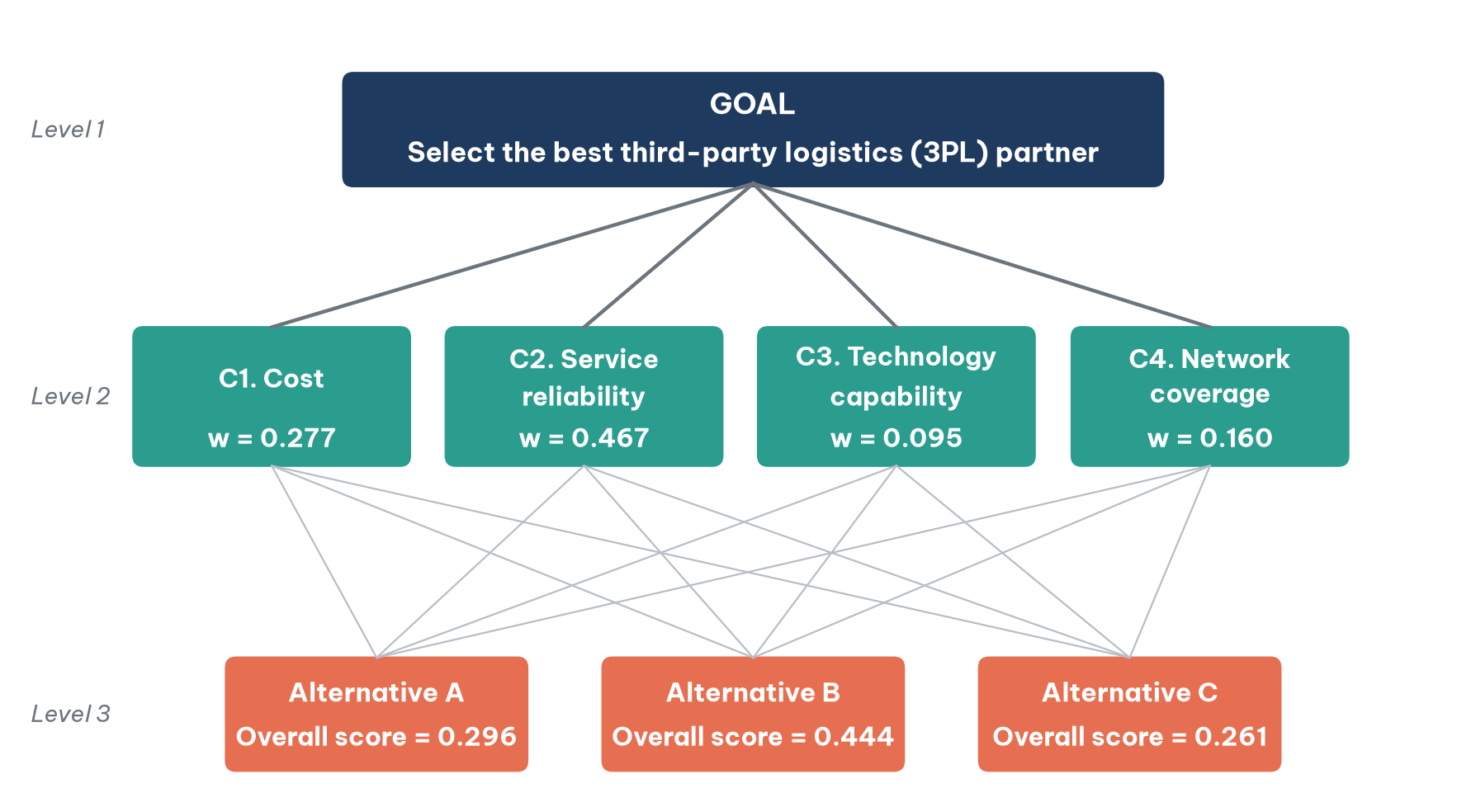
After discussions with purchasing, operations and finance, the decision team agrees on four criteria:
C1. Cost: total service cost over three years, including warehousing, transport and surcharges.
C2. Service reliability: on-time delivery rate, damage rate and ability to resolve incidents.
C3. Technology capability: warehouse management system (WMS), real-time shipment tracking and integration through EDI or APIs.
C4. Network coverage: the number of regions and delivery points the provider can serve.
The three bidders are labeled A, B and C. Figure 1 shows the three-level structure of the problem: the goal at the top, the four criteria in the middle and the three alternatives at the bottom, together with the weights and overall scores that the following steps will compute.
4.2. Step 2: compare the criteria in pairs
With four criteria, the team answers six comparison questions (4 × 3 / 2 = 6). Asked "How much more important is service reliability than cost?", the team judges reliability to be between equally and moderately more important and picks 2, reasoning that for food products a late shipment can cause losses far larger than any savings on freight. The resulting matrix is shown in Table 3.
4.3. Step 3: compute the weights and check consistency
Applying the approximation (divide each entry by its column total, then average across each row) gives weights of 0.277, 0.466, 0.096 and 0.161. The eigenvector method gives almost identical values, as Table 4 shows.
The largest eigenvalue is λmax = 4.031. Therefore CI = (4.031 − 4)/3 = 0.0103 and CR = 0.0103/0.90 = 0.0115, about 1.2%, far below the 10% threshold. The team's judgments are consistent.
What happens when judgments are inconsistent? Suppose another team member fills in the matrix with three cells changed: cost is moderately more important than reliability (3), reliability is more important than technology (4), yet technology is also judged more important than cost (2). All other cells stay as in Table 3. This is an intransitive loop: A beats B, B beats C, but C beats A. The calculation gives λmax = 5.203 and CR = 0.446, more than four times the acceptable threshold. AHP software flags such a matrix and points to the cells with the largest contradictions, helping the person see that they answered different questions from different frames of reference. This is one of the most practical benefits of AHP: it forces us to confront the inconsistencies in our own thinking.
4.4. Step 4: compare the alternatives under each criterion
Next, the team compares the bidders under each criterion. For cost, the question is "Which bidder is better (that is, cheaper), and by how much?" Quotations and capability documents inform the quantitative criteria; site visits and reference customers inform the qualitative ones. Table 5 gives the resulting local priorities and the consistency ratio of each matrix.
Table 5 makes the profile of each bidder plain: C is the cheapest, B is strongest on reliability and technology and A has the best network. All four matrices have a CR below 2%.
4.5. Step 5: synthesize and decide
Each bidder's overall score is the sum of the products of the criterion weights (Table 4) and its local priorities (Table 5). For bidder B:
P(B) = 0.277 × 0.122 + 0.467 × 0.648 + 0.095 × 0.625 + 0.160 × 0.297 ≈ 0.443
With the unrounded eigenvector weights, the same sum is 0.4438, or 0.444. Repeating the calculation for A and C gives the results in Table 6, computed from the unrounded weights. Using the rounded weights instead can shift the last digit by one, which is worth knowing when you check the arithmetic by hand.
Bidder B is clearly preferred. C, despite being the cheapest, ranks last because it is weak on reliability, the criterion with the highest weight. The result reflects the values the team declared and can be defended before the board: "We are not choosing B on instinct. Given the priorities we agreed on, B delivers the greatest overall value."
4.6. Group decisions: combining the judgments of several experts
Decisions are usually made by groups, and AHP offers two ways to combine views (Forman & Peniwati, 1998). The aggregation of individual judgments (AIJ) takes the geometric mean of the judgments in each cell; Aczél and Saaty (1983) proved that the geometric mean is the only rule that preserves the reciprocal property of the matrix. The aggregation of individual priorities (AIP) has each person compute their own weights and then averages them. AIJ suits a group acting as a single unit, AIP a group whose members represent separate stakeholders.
Suppose that in our example three experts (the head of purchasing, the head of operations and the chief accountant) each evaluate the criteria. The chief accountant puts more weight on cost (a cost weight of 0.383), while the head of operations emphasizes reliability (0.553). After aggregation with the geometric mean, the group weights are cost 0.272, reliability 0.455, technology 0.098 and network 0.175, with a CR of 0.013. The ranking does not change (B 0.441, A 0.300, C 0.259), which suggests that the decision is robust to the differences in view among team members.
4.7. Sensitivity analysis: is the conclusion robust?
A good decision must be able to answer the question "What if we got the weights slightly wrong?" Sensitivity analysis changes the weight of one criterion, rescales the others proportionally so that the weights still sum to 1 and watches how the ranking moves. Figure 2 plots the overall scores of the three bidders as the weight of cost runs from 0 to 0.9.
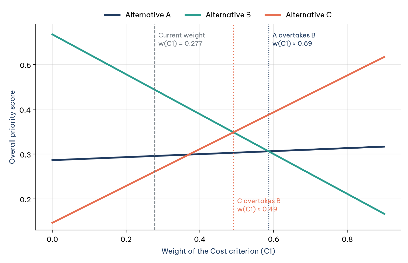
Figure 2 shows that B stays first until the weight of cost reaches about 0.49, roughly 1.8 times its current level of 0.277; beyond that, the cheapest bidder, C, moves ahead. Past about 0.59, A also overtakes B. (C passes A earlier, at about 0.37, but that only swaps second and third place.) Unless the company shifts to aggressive cost cutting, the choice of B is robust. Sensitivity analysis turns a static number into a strategic conversation and belongs in every serious AHP report.
5. When a hierarchy is not enough: the Analytic Network Process
This section shows when the independence assumption behind AHP breaks down, introduces ANP and extends the 3PL example into a network.
5.1. The limits of the independence assumption
AHP assumes that criteria are independent of one another and of the alternatives. Often they are not. In the 3PL example, a provider's technology directly affects its service reliability (good tracking reduces late deliveries) and its cost (automation lowers operating costs). A wide network also affects both cost and reliability. Furthermore, the set of available alternatives feeds back on which criteria we care about: if all three bidders quoted nearly the same price, cost would do little to separate them.
Saaty (2004b) describes ANP as a general framework for making decisions without assuming that upper-level elements are independent of lower ones or that elements within a level are independent of one another. ANP uses a network instead of a hierarchy and does not need to define levels.
5.2. Basic concepts of ANP
Six concepts appear in every ANP package and textbook:
Clusters and nodes: elements are grouped into clusters such as Criteria, Alternatives, Competitors or Customers.
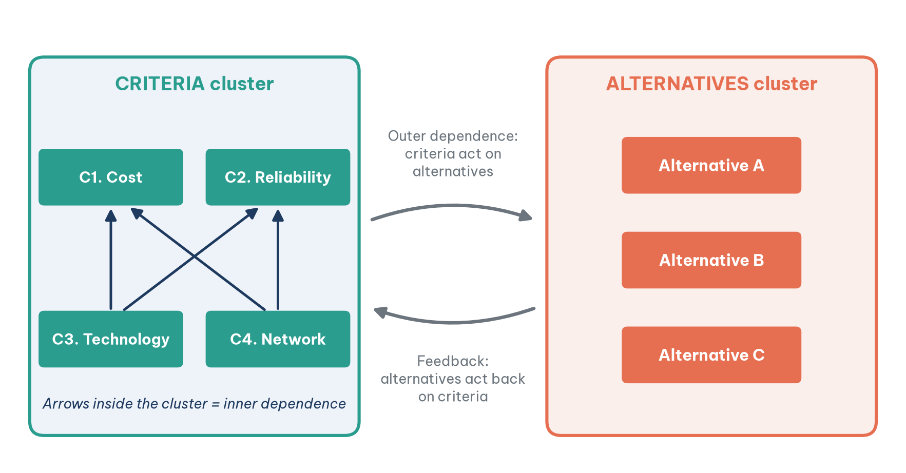
Outer dependence: nodes in one cluster influence nodes in another cluster.
Inner dependence: nodes within the same cluster influence one another, drawn as a loop on the cluster.
Feedback: influence runs in both directions between two clusters.
Supermatrix: a matrix holding all local priority vectors; each column shows the influence other nodes receive with respect to one node.
Control hierarchy and the BOCR model: for large problems, Saaty proposed building separate subnetworks for Benefits, Opportunities, Costs and Risks and then combining them (Saaty, 2004b; Saaty & Vargas, 2013).
Figure 3 shows these concepts on the 3PL problem: a Criteria cluster and an Alternatives cluster, inner-dependence arrows inside the Criteria cluster and a feedback loop between the two clusters.
5.3. How ANP is computed
The ANP procedure has four main steps, and the third is the biggest departure from AHP:
Build the network: define the clusters, the nodes and the lines of influence among them.
Make pairwise comparisons: for each "controlling" node, compare the nodes it influences within each cluster. The question is no longer "which is more important?" but "with respect to element X, how much more strongly does element A influence it than element B?"
Form the supermatrices:
The unweighted supermatrix places each local priority vector in its proper position.
The weighted supermatrix multiplies each block by the weight of its cluster (also obtained through pairwise comparison of clusters) so that every column sums to 1, making the matrix column stochastic.
The limit supermatrix raises the weighted supermatrix to large powers until its columns converge, capturing every chain of direct and indirect influence, much as a rumor spreads through layers of acquaintances.
Read the results: the final priorities of the alternatives (and of the criteria) are read from the limit supermatrix and then normalized within each cluster.
5.4. An ANP extension of the 3PL example
This subsection turns the AHP example into a network of seven nodes (four criteria and three alternatives) with three kinds of relationship:
Criteria act on alternatives: the four priority vectors from Table 5 are reused unchanged.
Alternatives feed back on criteria: for each bidder, the team asks "For this provider, which characteristic is its most distinctive strength?" For C, cost stands out most (0.467); for B, reliability (0.478) and technology (0.256) stand out.
Inner dependence among criteria: technology influences cost (0.4) and reliability (0.6); network influences cost and reliability equally (0.5 each).
In the columns for the criteria that have inner dependence (C3 and C4), the cluster weights are set at 0.3 for the Criteria cluster and 0.7 for the Alternatives cluster; every other column draws on a single cluster, which therefore takes the full weight of 1. Table 7 is the unweighted supermatrix. It is read by column: each column shows the influence the row nodes receive with respect to the node at the top of the column.
After the cluster weights are applied and the matrix is raised to powers until it converges, the results can be set beside those of AHP, as in Table 8.
Two results stand out. First, the ranking does not change, but B's lead over the runner-up widens from 0.148 to 0.174. Second, and more important, the weight of technology rises from 0.095 to 0.153. Asked directly, the team ranked technology last; once the model treats it as the engine behind reliability and cost efficiency, its real importance appears. This is the core value of ANP: it reveals indirect influence that intuition overlooks.
6. AHP and ANP compared
This section sets the two methods side by side after seeing both applied to the same problem, using the eight dimensions in Table 9.
The practical advice is to start with AHP and move to ANP only when interactions among criteria seem strong enough to change the conclusion. Sarkis et al. (2007) note that ANP demands a great deal of managerial input and readily tires decision makers.
7. AHP and ANP in practice
This section collects applications with published sources, grouped by field: large companies, health care, validation exercises with ANP and hybrid models in spatial planning and supply chains.
7.1. Large companies and high-stakes decisions
IBM and the AS/400. Saaty (2004a) recounts that IBM used AHP as part of its quality improvement strategy when designing the AS/400 computer line, a project that helped IBM win the Malcolm Baldrige National Quality Award. The story of the project is told in detail in The Silverlake Project (Bauer et al., 1992).
Billion-dollar decisions. Saaty (2008b) lists many specific applications. In 2001, AHP helped choose the site for rebuilding the Turkish city of Adapazari after an earthquake. In 1998, British Airways used it to choose an in-flight entertainment supplier for its whole fleet. In 1987, a company used it to choose the type of North Atlantic oil platform to build, a structure costing around US$3 billion, where decommissioning cost weighed even more heavily. Another corporation used AHP to allocate close to US$1 billion among research projects, and in 1999 Ford Motor Company used it to prioritize criteria for customer satisfaction.
Forman and Gass's catalog. Forman and Gass (2001) describe successful applications at Xerox, British Columbia Ferries, NASA (a propulsion system for a lunar lander), General Motors, the U.S. Federal Aviation Administration and the U.S. Navy's submarine operations. They also note that the American Society for Testing and Materials (ASTM) adopted AHP as a standard practice for multi-attribute analysis of building-related investments.
Selecting a telecommunications vendor. Tam and Tummala (2001) applied AHP to a real choice of telecommunications system vendor involving decision makers from several departments with conflicting objectives. The model improved group decision making, made the process more systematic and shortened the time needed to select a vendor.
Project portfolios and marketing. At the Project Management Institute (PMI) Global Congress in 2010, Vargas (2010) showed how to use AHP to select and prioritize the projects in a portfolio so that it flows from the organization's strategic objectives. Much earlier, Wind and Saaty (1980) illustrated AHP in marketing decisions such as choosing target products, markets and channels, evaluating new product ideas and setting the marketing mix.
7.2. Health care
Health care decisions involve many stakeholders and hard-to-quantify criteria, and AHP has attracted several systematic reviews there. Liberatore and Nydick (2008) reviewed 50 articles applying AHP in medicine and health care and sorted them into seven groups: diagnosis, patient participation, therapy and treatment, organ transplantation, project and technology evaluation and selection, human resource planning and health care evaluation and policy. The largest group was technology evaluation and selection (14 articles), followed by patient participation (9 articles). The authors saw AHP as a promising tool for shared decision making between clinicians and patients.
Another systematic review, by Hummel and IJzerman (2009), found 57 applications of AHP in health care, of which 44% concerned management decisions within health care organizations and 25% concerned the development of clinical practice guidelines.
7.3. ANP for estimation: when judgment matches real data
Some of the most persuasive evidence for AHP and ANP comes from validation exercises, in which results derived from judgment are compared with known actual figures. Rozann Whitaker (2007), who also publishes as Rozann W. Saaty, compiles many such exercises. A striking example estimates the market shares of the U.S. breakfast cereal industry with ANP, using only judgments about competitive factors and no sales data (Table 10).
The compatibility index between the two vectors in Table 10 is about 1.01, very close to the ideal value of 1 and below the threshold of 1.1 that Saaty commonly uses to treat two priority vectors as close. Saaty (2004b) presents a similar exercise with the market shares of three U.S. retail chains, Walmart, Kmart and Target.
ANP has also been applied to crises and operations. Saaty and Vargas (2013) devote a chapter to the Ford Explorer case after the August 2000 recall of 6.5 million Firestone tires, weighing responses in which brand image, public image and economic risk influenced one another. Meade and Sarkis (1999), among the first to use ANP in operations management, evaluated projects to make a small real manufacturer more agile.
7.4. Hybrid models: evidence from spatial planning and supply chains
Outside the classic corporate cases, much of today's applied work uses AHP inside hybrid models, combined with geographic information systems (GIS), fuzzy sets, data envelopment analysis (DEA) or TOPSIS. A cluster of recent studies from Vietnam, a fast-growing economy facing pressure on land, waste systems and supply chains at the same time, shows the pattern clearly.
Landfill siting with GIS. Oanh et al. (2024) combined GIS with AHP, using national siting standards as exclusion criteria, to assess land for a solid waste landfill in a peri-urban district of Hanoi, where an existing facility had run into trouble because of a poorly chosen site. Only 220.89 hectares (1.18%) of the study area proved suitable, against 56.81% unsuitable and 42.01% marginally suitable. In the environmentally sensitive Mekong Delta, Nguyen et al. (2022) built a nine-criterion GIS and AHP model for Ben Tre Province that added geological criteria such as soil type, permeability and soil thickness. Nguyen et al. (2025) went a step further and integrated GIS with fuzzy AHP for Phu Yen Province on the central coast: 45% of the study area had high or very high potential, 28% moderate and 27% low or very low, and, notably, 25.7% of existing landfills were located where they posed significant environmental risk.
Supplier selection. Wang et al. (2018a) combined fuzzy ANP with DEA to select suppliers in a rice supply chain, with fuzzy ANP ranking the criteria that drive profitability. Wang et al. (2018b) paired fuzzy AHP, which set criterion weights from purchasing experts' views, with a green DEA model that ranked edible oil suppliers for small food processors. Wang et al. (2022) combined fuzzy AHP and fuzzy TOPSIS to rank ten leading steel producers as green suppliers on price, quality, delivery, service and environmental performance.
These studies show a clear trend: AHP is seldom used alone in such settings and is far more often hybridized (fuzzy AHP, AHP with GIS, ANP with DEA, AHP with TOPSIS). The trend matches the observation by Emrouznejad and Marra (2017) that integrated AHP models have grown rapidly worldwide.
8. Debates and limitations to know
No method is perfect. This section covers the five issues raised most often, which professional users of AHP and ANP need to understand in order to apply the methods in the right place and report their results honestly.
8.1. Rank reversal
The best-known debate concerns rank reversal. Belton and Gear (1983) showed that adding a new alternative, even an exact copy of an existing one, can reverse the ranking of the original alternatives. Dyer (1990) went further and argued that this makes AHP results potentially arbitrary; Saaty (1990b) replied in the same issue of the journal.
A simple example shows the effect. Three alternatives, A, B and C, receive raw scores on three equally weighted criteria: A = (1, 9, 8), B = (9, 1, 9) and C = (1, 1, 1). With the usual normalization (the distributive mode, which divides each score by the column total), the overall scores are A = 0.451 and B = 0.470, so B ranks above A. Now add an alternative B′ identical to B. The new scores are A = 0.365 and B = B′ = 0.289, so A now ranks above B, even though nothing about the assessment of A or B has changed.
The distributive mode shares value among alternatives, so a copy of B splits B's share on the criteria where it is strong. Saaty and Vargas (2012) argue that rank reversal is an inherent property of relative measurement and can be legitimate in some contexts, for example when scarcity adds value. When rank must be preserved, one can use the ideal mode (dividing by the largest value in each column) or absolute measurement with ratings. In the example above, the ideal mode gives A = 0.667 and B = 0.704 (average scores before final normalization) both before and after B′ is added, so the ranking is preserved.
The practical lesson is to choose the synthesis mode deliberately. If you are choosing one best alternative and the set of alternatives may change, the ideal mode is usually safer. If you are allocating a scarce resource in proportion to priorities, the distributive mode may be more appropriate.
8.2. The comparison burden
Comparisons grow with the square of the number of elements: 9 criteria need 36, and an ANP model can need hundreds. Fatigue degrades judgment. Remedies include multi-level structures, absolute ratings for many alternatives and incomplete comparison matrices.
8.3. The fuzzy AHP debate
Fuzzy AHP, which grew out of Buckley (1985) and the extent analysis method of Chang (1996), is popular in applied research, including several studies in Section 7.4. Saaty opposed it. Saaty and Tran (2007) argue that 1–9 judgments are already fuzzy, that fuzzifying them further has no theoretical basis and that it can move results away from known answers. Researchers who use fuzzy AHP should acknowledge this debate and justify their choice.
8.4. Garbage in, garbage out
AHP and ANP do not create truth out of nothing. Results depend on a complete structure, genuinely knowledgeable experts and clearly worded questions. A structure that omits an important criterion will produce results that are perfectly consistent and dangerously wrong.
8.5. Cognitive biases do not disappear
Breaking judgments into small pieces reduces cognitive bias but does not remove it. Anchoring occurs when a facilitator suggests a number first; groupthink occurs when members fill in matrices in front of their superiors. Have each member answer independently, discuss the largest differences, then aggregate with the geometric mean.
9. A ten-step procedure for practice
This section distills the example and the debates above into a ten-step procedure for AHP and ANP projects in business and applied research:
Define the decision goal in one specific sentence with a time frame.
Assemble a cross-functional panel of 5 to 10 people representing those affected by the decision.
Build the list of criteria from the literature, expert interviews and experience, checking that criteria do not overlap and can be assessed.
Design the hierarchy or network. Keep each comparison group to 7 elements or fewer. If you suspect strong interactions among criteria, consider ANP, or use DEMATEL first to map the structure of influence.
Design the questionnaire with clear questions, examples of the 1–9 scale and the direction of each criterion (for instance, "lower cost is better").
Collect judgments independently from each expert.
Compute the weights and check CR for every matrix; where CR exceeds 0.10, review the most contradictory cells with the expert.
Aggregate the group's views with the geometric mean of judgments (AIJ) or by averaging priorities (AIP), depending on the nature of the group.
Synthesize and run sensitivity analysis. Identify the points at which the ranking changes and check whether the conclusion holds under reasonable changes in the weights.
Present and justify. Report not only the final numbers but also the structure, the weights, the CR values and the sensitivity results. State the synthesis mode used (distributive or ideal).
On tools: for small problems, a spreadsheet with the approximation method is entirely adequate. For large problems or ANP, use specialized software such as Expert Choice or Super Decisions, or write your own code in Python or R; all you need is a linear algebra library to compute eigenvectors and matrix powers.
10. When to use AHP and ANP, and when not to
AHP and ANP cost expert time and require a disciplined process, so not every decision deserves them. This section sets out where they pay off. They are worth using when:
The decision involves several conflicting criteria, including qualitative ones that are hard to measure.
The views of several stakeholders must be gathered and combined transparently.
The decision must be justified to a board, shareholders or a regulator.
Quantitative data is incomplete but knowledgeable experts are available.
The decision has large and lasting consequences, enough to justify a structured process.
Consider other methods in three situations:
The number of alternatives is very large (dozens or hundreds). AHP can still set the criterion weights, while TOPSIS, VIKOR or absolute ratings rank the alternatives.
Every criterion has objective quantitative data. Methods such as DEA or multi-objective optimization may fit better.
The decision must be made very quickly, or it is an operational choice repeated every day.
Conclusion
More than four decades after they were introduced, AHP and ANP remain among the most widely used methods for multi-criteria decisions, from the boardrooms of IBM, Ford and British Airways to landfill siting studies in rapidly urbanizing regions. Their strength lies less in mathematics than in their ability to turn subjective judgments into disciplined numbers: break the problem apart, compare its pieces two at a time, check your own consistency and test whether the conclusion holds.
The worked example showed AHP taking a management team from opinion-driven debate to a choice it can defend (bidder B, with a score of 0.444), and sensitivity analysis showed how far the weights would have to move before that choice changed. ANP added a further insight: technology capability matters far more than the team first believed, because of its indirect role in driving reliability and cost. At the same time, the debates over rank reversal, the comparison burden and fuzzy AHP are reminders that every tool must be used with understanding and intellectual honesty.
As Saaty (2008a) emphasized, decision making has become a science, and AHP and ANP help formalize the way we already think so that every aspect of a decision becomes visible. For managers, analysts and researchers, mastering the two methods is less about adding another analytical technique than about building the habit of structured thinking before the choices that matter most.
References
Aczél, J., & Saaty, T. L. (1983). Procedures for synthesizing ratio judgements. Journal of Mathematical Psychology, 27(1), 93–102. https://doi.org/10.1016/0022-2496(83)90028-790028-7)
Bauer, R. A., Collar, E., & Tang, V. (1992). The Silverlake Project: Transformation at IBM. Oxford University Press. https://www.amazon.com/s?k=The+Silverlake+Project+Bauer&i=stripbooks
Belton, V., & Gear, T. (1983). On a short-coming of Saaty's method of analytic hierarchies. Omega, 11(3), 228–230. https://doi.org/10.1016/0305-0483(83)90047-690047-6)
Buckley, J. J. (1985). Fuzzy hierarchical analysis. Fuzzy Sets and Systems, 17(3), 233–247. https://doi.org/10.1016/0165-0114(85)90090-990090-9)
Chang, D.-Y. (1996). Applications of the extent analysis method on fuzzy AHP. European Journal of Operational Research, 95(3), 649–655. https://doi.org/10.1016/0377-2217(95)00300-200300-2)
Dyer, J. S. (1990). Remarks on the analytic hierarchy process. Management Science, 36(3), 249–258. https://doi.org/10.1287/mnsc.36.3.249
Emrouznejad, A., & Marra, M. (2017). The state of the art development of AHP (1979–2017): A literature review with a social network analysis. International Journal of Production Research, 55(22), 6653–6675. https://doi.org/10.1080/00207543.2017.1334976
Forman, E., & Peniwati, K. (1998). Aggregating individual judgments and priorities with the analytic hierarchy process. European Journal of Operational Research, 108(1), 165–169. https://doi.org/10.1016/S0377-2217(97)00244-000244-0)
Forman, E. H., & Gass, S. I. (2001). The analytic hierarchy process: An exposition. Operations Research, 49(4), 469–486. https://doi.org/10.1287/opre.49.4.469.11231
Hummel, J. M., & IJzerman, M. J. (2009). A systematic review of the analytic hierarchy process in health care decision making [Conference abstract]. Value in Health, 12(7). https://www.ispor.org/heor-resources/presentations-database/presentation/ispor-12th-annual-european-congress/a-systematic-review-of-the-analytic-hierarchy-process-in-health-care-decision-making
Institute for Operations Research and the Management Sciences. (n.d.). Dr. Thomas L. Saaty. Retrieved November 18, 2026, from https://www.informs.org/Recognizing-Excellence/Award-Recipients/Dr.-Thomas-L.-Saaty
Liberatore, M. J., & Nydick, R. L. (2008). The analytic hierarchy process in medical and health care decision making: A literature review. European Journal of Operational Research, 189(1), 194–207. https://doi.org/10.1016/j.ejor.2007.05.001
Meade, L. M., & Sarkis, J. (1999). Analyzing organizational project alternatives for agile manufacturing processes: An analytical network approach. International Journal of Production Research, 37(2), 241–261. https://doi.org/10.1080/002075499191751
Nguyen, D.-M. T., Robinson, D. T., Zurbrügg, C., Nguyen, T. H. T., Dang, H.-L., & Pham, V.-M. (2025). Strategic landfill site selection for sustainable waste management in Phu Yen Province, Vietnam using geospatial technologies. Ecological Informatics, 89, Article 103198. https://doi.org/10.1016/j.ecoinf.2025.103198
Nguyen, D.-T., Truong, M.-H., Ngo, T.-P.-U., Le, A.-M., & Yamato, Y. (2022). GIS-based simulation for landfill site selection in Mekong Delta: A specific application in Ben Tre Province. Remote Sensing, 14(22), Article 5704. https://doi.org/10.3390/rs14225704
Oanh, N. T., Thanh, P. T., Long, N. B., Chien, L. H., Dinh, N. T., Thom, T. T., Bich, N. T., & Elshewy, M. A. (2024). Optimal solid waste landfill site identification employing GIS-based multi-criteria decision analysis within the Thach That District, Hanoi, Vietnam. International Journal of Geoinformatics, 20(1). https://doi.org/10.52939/ijg.v20i1.3021
Saaty, T. L. (1977). A scaling method for priorities in hierarchical structures. Journal of Mathematical Psychology, 15(3), 234–281. https://doi.org/10.1016/0022-2496(77)90033-590033-5)
Saaty, T. L. (1980). The analytic hierarchy process: Planning, priority setting, resource allocation. McGraw-Hill. https://www.amazon.com/s?k=The+analytic+hierarchy+process+Saaty&i=stripbooks
Saaty, T. L. (1990a). How to make a decision: The analytic hierarchy process. European Journal of Operational Research, 48(1), 9–26. https://doi.org/10.1016/0377-2217(90)90057-I90057-I)
Saaty, T. L. (1990b). An exposition of the AHP in reply to the paper "Remarks on the analytic hierarchy process." Management Science, 36(3), 259–268. https://doi.org/10.1287/mnsc.36.3.259
Saaty, T. L. (1996). Decision making with dependence and feedback: The analytic network process. RWS Publications. https://www.amazon.com/s?k=Decision+making+with+dependence+and+feedback+Saaty&i=stripbooks
Saaty, T. L. (2004a). Decision making: The analytic hierarchy and network processes (AHP/ANP). Journal of Systems Science and Systems Engineering, 13(1), 1–35. https://doi.org/10.1007/s11518-006-0151-5
Saaty, T. L. (2004b). Fundamentals of the analytic network process: Dependence and feedback in decision-making with a single network. Journal of Systems Science and Systems Engineering, 13(2), 129–157. https://doi.org/10.1007/s11518-006-0158-y
Saaty, T. L. (2008a). Decision making with the analytic hierarchy process. International Journal of Services Sciences, 1(1), 83–98. https://doi.org/10.1504/IJSSCI.2008.017590
Saaty, T. L. (2008b). Relative measurement and its generalization in decision making. Why pairwise comparisons are central in mathematics for the measurement of intangible factors: The analytic hierarchy/network process. RACSAM: Revista de la Real Academia de Ciencias Exactas, Físicas y Naturales. Serie A. Matemáticas, 102(2), 251–318. https://doi.org/10.1007/BF03191825
Saaty, T. L., & Ozdemir, M. S. (2003). Why the magic number seven plus or minus two. Mathematical and Computer Modelling, 38(3–4), 233–244. https://doi.org/10.1016/S0895-7177(03)90083-590083-5)
Saaty, T. L., & Tran, L. T. (2007). On the invalidity of fuzzifying numerical judgments in the analytic hierarchy process. Mathematical and Computer Modelling, 46(7–8), 962–975. https://doi.org/10.1016/j.mcm.2007.03.022
Saaty, T. L., & Vargas, L. G. (2012). The seven pillars of the analytic hierarchy process. In T. L. Saaty & L. G. Vargas (Eds.), Models, methods, concepts & applications of the analytic hierarchy process (2nd ed., pp. 23–40). Springer. https://doi.org/10.1007/978-1-4614-3597-6_2
Saaty, T. L., & Vargas, L. G. (2013). Decision making with the analytic network process: Economic, political, social and technological applications with benefits, opportunities, costs and risks (2nd ed.). Springer. https://doi.org/10.1007/978-1-4614-7279-7
Sarkis, J., Talluri, S., & Gunasekaran, A. (2007). A strategic model for agile virtual enterprise partner selection. International Journal of Operations & Production Management, 27(11), 1213–1234. https://doi.org/10.1108/01443570710830601
Tam, M. C. Y., & Tummala, V. M. R. (2001). An application of the AHP in vendor selection of a telecommunications system. Omega, 29(2), 171–182. https://doi.org/10.1016/S0305-0483(00)00039-600039-6)
Vaidya, O. S., & Kumar, S. (2006). Analytic hierarchy process: An overview of applications. European Journal of Operational Research, 169(1), 1–29. https://doi.org/10.1016/j.ejor.2004.04.028
Vargas, R. V. (2010). Using the analytic hierarchy process (AHP) to select and prioritize projects in a portfolio [Paper presentation]. PMI Global Congress 2010, North America, Washington, DC, United States. https://www.pmi.org/learning/library/analytic-hierarchy-process-prioritize-projects-6608
Wang, C.-N., Nguyen, T.-L., & Dang, T.-T. (2022). Two-stage fuzzy MCDM for green supplier selection in steel industry. Intelligent Automation & Soft Computing, 33(2), 1245–1260. https://doi.org/10.32604/iasc.2022.024548
Wang, C.-N., Nguyen, V. T., Duong, D. H., & Do, H. T. (2018a). A hybrid fuzzy analytic network process (FANP) and data envelopment analysis (DEA) approach for supplier evaluation and selection in the rice supply chain. Symmetry, 10(6), Article 221. https://doi.org/10.3390/sym10060221
Wang, C.-N., Nguyen, V. T., Thai, H. T. N., Tran, N. N., & Tran, T. L. A. (2018b). Sustainable supplier selection process in edible oil production by a hybrid fuzzy analytical hierarchy process and green data envelopment analysis for the SMEs food processing industry. Mathematics, 6(12), Article 302. https://doi.org/10.3390/math6120302
Whitaker, R. (2007). Validation examples of the analytic hierarchy process and analytic network process. Mathematical and Computer Modelling, 46(7–8), 840–859. https://doi.org/10.1016/j.mcm.2007.03.018
Wind, Y., & Saaty, T. L. (1980). Marketing applications of the analytic hierarchy process. Management Science, 26(7), 641–658. https://doi.org/10.1287/mnsc.26.7.641
Discussion about this post