A/B Testing from Hypothesis to Conclusion
A trustworthy A/B test starts with a clear hypothesis and enough data, not with the testing tool


Key takeaways
Write the hypothesis, the primary metric and the minimum effect worth detecting before the test starts.
Sample size grows with the inverse square of the effect you want to detect: halving the effect needs four times the data.
Run whole weeks, do not stop the moment p drops below 0.05, and check for sample ratio mismatch.
Testing one factor at a time is slow and misses interactions; factorial designs test several factors in one campaign.
Read results through confidence intervals translated into money, and treat segment "wins" as hypotheses for the next test.
An online shop changes its "Buy now" button from grey to orange, runs the test for three days and sees orders rise by 15%. The team celebrates and rolls the change out across the site. A month later, sales look exactly as before. Nobody got a formula wrong. Three days was simply too short, a 15% rise was within the range of random noise, and the test week happened to coincide with payday. An A/B test sounds simple: split customers into two groups, show each group a different version, compare the results. But between that simple idea and a trustworthy conclusion lie many small decisions, and each wrong one can turn a test into an expensive coin toss.
This article is about the practice: how to make an A/B test in business actually answer the question it was meant to answer. It draws heavily on the chapter on the "test and learn" strategy in Haughton et al. (2026), combined with the lessons from large-scale online experimentation summarized by Kohavi et al. (2020).
The article has eight parts. Section 1 introduces A/B testing and its place in the test-and-learn cycle. Section 2 covers writing hypotheses and choosing metrics. Section 3 explains sample size and test duration. Section 4 deals with assigning groups, including blocked randomization and sample ratio checks. Section 5 extends to testing several factors at once with factorial designs. Section 6 shows how to read results. Section 7 lists seven common mistakes, and Section 8 surveys tools.
1. A/B testing and the test-and-learn cycle
An A/B test compares two options: the current version (the control group, usually called A) and a new version (the treatment group, B). Each customer or visit is randomly assigned to one group. Because assignment is random, the two groups are alike in every respect, including things we cannot measure such as mood or how rushed people are, so any difference in outcomes can be attributed to the change itself. Group A plays the role of "what would have happened without the change", something we can never observe directly for the same customer.
1.1. From A/B to A/B/n
When there are more than two versions of the same factor, say three price points or four email subject lines, the test is called A/B/n. The principle is unchanged: one random group per version, all running over the same period. What matters is that an A/B test isolates the effect of one factor. Haughton et al. (2026) give the example of a shoe retailer testing a new message about versatility against the old message about durability, while also lowering the price for the new-message group. If the new group sells more, nobody can tell whether the message or the price did it. Separating the two effects requires the designs in Section 5.
1.2. A test is one step in a larger cycle
An A/B test rarely stands alone. Haughton et al. (2026) place it within a seven-step "test and learn" strategy that marketers use widely even though textbooks seldom discuss it. Figure 1 shows the cycle: it starts with the voice of the customer (qualitative research, surveys) and the voice of the industry (competitor and market analysis), derives business opportunities and goals, lists the value propositions to test, and only then moves to test, measure and learn. What is learned feeds the next round.
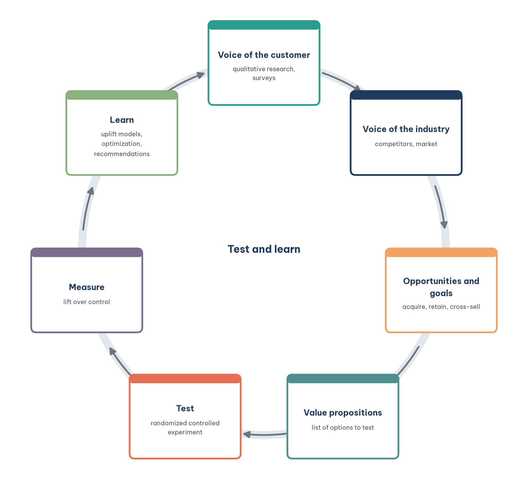
The cycle is a reminder of something often overlooked: the list of options to test should come from understanding customers, not from the preferences of the most senior person in the meeting. A team that runs dozens of button-color tests without understanding why customers abandon their carts is busy but learns nothing.
2. Start with a hypothesis and a metric
Before touching any tool, write down two things: the hypothesis and the metric. Together they determine how much data the test needs, how long it runs and how the result is read. Writing them down first also blocks a dangerous habit: running the test and then looking for whichever metric looks good.
2.1. Write the hypothesis as a testable sentence
A good hypothesis has three parts: what changes, which metric is expected to move and by how much, and why. For example: "If delivery fees are shown on the product page instead of at checkout, the order completion rate will rise by at least 10%, because surveys show many customers abandon their carts when surprised by the fee." The "why" connects the test to customer insight; "at least 10%" is the minimum effect of interest, used to compute sample size in Section 3. A hypothesis such as "the new design will be better" cannot be tested, because it says neither where nor by how much.
2.2. Choose a primary metric, secondary metrics and guardrails
Each test should have one primary metric, tied directly to the business goal and chosen in advance. Alongside it sit a few secondary metrics that explain the mechanism, and guardrail metrics that make sure the new version does no harm elsewhere, such as page load time, return rates or complaint calls. Kohavi et al. (2020) call the overall primary metric the "overall evaluation criterion" and urge companies to invest time in agreeing on it, because a short-term metric such as clicks can rise while long-term customer value falls.
Haughton et al. (2026) organize metrics along the AIDA funnel (awareness, interest, desire, action) and make an important point: every metric has two versions, the baseline (for example the purchase rate in the treatment group) and the lift (the treatment purchase rate minus the control purchase rate). Only the lift measures the effect of the campaign. Table 1 summarizes common metrics and their roles.
Table 1 shows that the further down the funnel, the closer a metric is to the real goal, but the rarer and noisier it becomes, so the more data it needs. That is why many teams pick a mid-funnel metric such as click-through as the primary metric. This is acceptable if there is evidence that the mid-funnel metric actually leads to the bottom-funnel one; without it, the test may optimize something that does not matter.
3. Sample size and test duration
The question "how long should we run it?" is a question about sample size, and sample size must be computed before the test begins, not when the result already looks "significant". This section explains the four quantities that determine sample size and how to convert it into days.
3.1. Two kinds of error and statistical power
Every statistical test can go wrong in two ways. A Type I error is concluding the new version is better when it is not; its probability is the significance level α, usually set at 5%. A Type II error is missing an improvement that is real; its probability is β, and 1 − β is the power of the test, usually set at 80%. A lower α and higher power give a more reliable conclusion but require more data.
The other two quantities are the baseline rate of the control group (from historical data) and the minimum detectable effect, the "at least 10%" in the hypothesis. The last one matters most: sample size is inversely proportional to the square of the difference, so detecting an effect half as large needs four times as much data. Table 2 illustrates this for a baseline conversion rate of 3%, a two-sided 5% significance level and 80% power.
Table 2 explains the story at the start of this article. A small site with 2,000 visits a day can hardly detect a 5% lift in any reasonable time. If the business only cares about large changes (20% or more), two weeks is enough; if it wants to fine-tune every small detail, it needs the traffic of a major marketplace. Knowing this in advance helps a team test changes that are bold enough instead of changing button colors.
The calculation in Table 2 takes a few lines of Python. The code below computes the sample size per group needed to detect a rise from 3% to 3.6%:
from scipy.stats import norm

def sample_size(p_a, p_b, alpha=0.05, power=0.8):
    z_a = norm.ppf(1 - alpha / 2)
    z_b = norm.ppf(power)
    variance = p_a * (1 - p_a) + p_b * (1 - p_b)
    return (z_a + z_b) ** 2 * variance / (p_b - p_a) ** 2

print(round(sample_size(0.03, 0.036)))
The output is 13,911 customers per group. When there is no history from which to estimate the baseline rate, Haughton et al. (2026) suggest running the calculation over a reasonable range of values and choosing the largest sample size in that range.
3.2. From sample size to duration, and why not to stop early
With the sample size in hand, divide by daily traffic to get the number of days, then round up to whole weeks. Shopping behavior differs between weekdays and weekends, and between the start and end of the month; running in whole weeks lets both groups experience the full cycle. Also avoid special periods such as major holidays, Black Friday or a big promotion, unless that period is itself what you want to test.
The most common mistake is peeking continuously and stopping as soon as the result is significant. If you check every day and stop the first time the p-value drops below 0.05, the real probability of a false conclusion is far higher than 5%, because chance has been given many opportunities to produce a "good" day. If the organization needs early monitoring, use sequential testing methods designed for repeated looks rather than the ordinary test.
Another phenomenon that distorts short-term results is the novelty effect: regular users click on a new design simply because it is new, then return to their old behavior a few weeks later. Conversely, some changes take time for users to get used to. Tracking the difference week by week helps spot both.
4. Assigning groups properly
Random assignment is the foundation of a test, and also where things quietly break. This section covers the unit of randomization, blocked randomization for small samples, and a simple check for broken assignment.
4.1. Choose the unit of randomization
The unit randomized can be a visit, a user, a store or a region. The principle is to choose a unit such that no one accidentally sees both versions. If you randomize by visit, the same customer might see price A in the morning and price B in the afternoon, which is both annoying and lets the groups contaminate each other. For price or policy tests, randomize by user; for in-store changes, the unit is the store. When the unit is a store or region, the number of units is usually small, and the technique in Section 4.2 is needed.
4.2. Blocked randomization for small samples
Haughton et al. (2026) give the example of a retail chain with 1,000 stores across the 50 US states that wants to test blue instead of yellow as its theme color (walls, staff uniforms) in 20 pilot stores. If the 10 blue stores are chosen completely at random, they may cluster in one region, and the sales difference would reflect regional differences rather than color. The solution is a randomized block design (also called stratified randomization): divide the stores into four regions, then randomly assign blue or yellow within each region. If the test must run over three months, month can be added as a blocking variable, giving 12 blocks.
The same logic applies to any chain testing a new menu or layout in a handful of outlets: block by region and by location type (office district, residential area), then randomize within each block. The technique is especially useful when units are few; with hundreds of thousands of online users, simple randomization already balances the groups.
4.3. Check for sample ratio mismatch
If the design splits traffic 50:50 but the result is 50,000 users in group A and 48,500 in group B, there may be a technical fault: version B loads slowly so some users leave before being logged, or the bot filter behaves differently between the groups. This is called sample ratio mismatch (SRM). Fabijan et al. (2019) show that SRM occurs quite often in online experiments and almost always signals an untrustworthy result. The check is simple: a chi-square test comparing the observed counts with the designed ratio. If there is SRM, do not analyze further; find the cause first. SRM combined with differences in group composition can even reverse a conclusion, as in Simpson's paradox.
5. Testing several factors at once
When several factors need testing, the natural approach is one at a time: price this month, fee next month, content the month after. This section explains why that approach is slow and can miss the best option, and how factorial designs solve the problem.
5.1. Why one factor at a time is not enough
Testing one factor at a time takes a long time, especially for direct mail campaigns that need weeks per round. More seriously, it implicitly assumes the factors do not affect one another: the best price from round one is held fixed when the fee is tested in round two. If the effect of the fee depends on the price, you may never find the best combination (Haughton et al., 2026). A design that tests every factor in a single campaign is known in business as multivariate testing. US credit card issuers have used this approach since the 1990s, and many card offers that households receive in the mail are actually one cell of a large experiment.
5.2. Factorial designs and interaction effects
The example from Haughton et al. (2026) is an airline selling a premium membership at $99 a year that cuts average check-in time by 5 minutes. The airline wants to know whether customers would pay more to be faster, so it tests two fee levels ($69 and $99) and two time reductions (5 and 15 minutes). A full factorial design has 2 × 2 = 4 cells, with customers randomly assigned to each. Table 3 shows one possible result.
Three effects can be computed from these four cells. The main effect of the fee is the average of the two high-fee cells minus the average of the two low-fee cells: (3% + 2%)/2 − (6% + 3%)/2 = −2 percentage points. The main effect of time is (6% + 3%)/2 − (3% + 2%)/2 = +2 points. The interaction effect tells whether the effect of one factor depends on the level of the other: with a 5-minute reduction, a lower fee adds only 1 point (3% versus 2%); with a 15-minute reduction, it adds 3 points (6% versus 3%). Figure 2 shows this as two non-parallel lines.
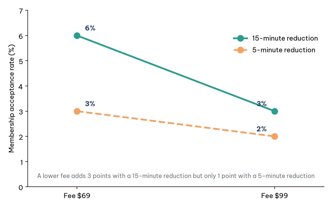
The business meaning of Figure 2 is that the two changes reinforce each other: customers are truly price-sensitive only when the benefit is large enough. Had the airline tested one factor at a time (first the fee at 5 minutes, then the time at the chosen fee), it would have underestimated the effect of a lower fee. A factorial design is also more efficient: every participant contributes information on both factors, so the total sample is smaller than for two separate tests.
5.3. When there are too many combinations: fractional factorial designs
The number of cells grows quickly. A retailer testing three factors at two levels each (a 20% or 30% discount, mailing once or twice a month, postcard or letter) already has 2³ = 8 cells. A bank testing interest rate, annual fee, benefits and card color, each at several levels, may face hundreds of combinations. A fractional factorial design runs only a systematically chosen subset of combinations, sacrificing some higher-order interactions (usually less important) while still estimating the main effects.
The key concept is the resolution of the design. In a resolution III design, main effects are not confounded with each other but may be confounded with two-factor interactions. In a resolution IV design, main effects are not confounded with two-factor interactions, but two-factor interactions may be confounded with each other. In practice, designs are generated by software (SAS, JMP, R), business constraints such as "never combine the lowest rate with a zero fee" can be added, and the design is then checked to confirm that all required effects are estimable (Haughton et al., 2026). A practical rule for beginners: if there is a business reason to suspect two factors interact (price and quality, say), choose a design that can estimate that interaction.
6. Reading the results
Once the test has run for its planned duration, reading the result involves three questions: is the difference larger than random variation, how large is it, and is it worth acting on? This section works through each with an example.
6.1. p-values and confidence intervals
Suppose each group has 15,000 customers; group A has 450 orders (3.0%) and group B has 540 (3.6%). A two-proportion test gives z ≈ 2.91 and a p-value ≈ 0.004. The p-value means: if the two versions were actually the same, the probability of seeing a difference this large or larger would be about 0.4%. It does not mean "there is a 99.6% probability that B is better". More useful is the 95% confidence interval of the difference: roughly 0.2 to 1.0 percentage points. It says B is better, but the improvement could be a modest 0.2 points or as large as 1 point.
6.2. Statistical significance and business significance
Statistical significance only says a difference is unlikely to be due to chance; it does not say the difference is worth the money. With very large samples, a lift of 0.01 percentage points can be "significant" without covering the cost of implementation. So translate the confidence interval into money: if each order earns $4 in profit and a million customers visit each month, a 0.2-point lift means 2,000 extra orders and $8,000 a month; if the cost of implementing and maintaining the new version is well below the figure at the lower end of the interval, the decision is fairly safe. Following Table 1, the final decision metric should be incremental revenue or ROI, not just the conversion rate.
6.3. Be careful when slicing by segment
After seeing the overall result, everyone wants to look by segment: new versus returning customers, mobile versus desktop, region by region. This helps understand the mechanism, but each slice is a new test, and with 20 segments one of them is almost certain to look "significant" by chance. Segment findings should be treated as hypotheses for the next test, unless the segment was specified in advance and the sample size computed for it. To exploit "which version suits whom" systematically requires uplift modeling, which estimates the effect of a treatment for each individual.
7. Seven common mistakes
Most tests fail not because a formula is wrong but because the process is. Table 4 summarizes the seven most frequent mistakes, how to spot them and how to avoid them.
Beyond these technical mistakes, there is an ethical one: testing on customers changes that could harm them, such as prices discriminating on personal characteristics or fear-based messages. Facebook's 2014 emotional contagion experiment remains the best-known warning. A methodologically sound test that destroys customer trust is still a failed test.
8. Tools
Tools only execute the decisions described above; they do not make them. Tools fall into three groups by role.
The first group is experimentation platforms that handle assignment, display of versions and logging on a website or app, such as Optimizely, VWO, or open-source options such as GrowthBook. Google Optimize, a once-popular free tool, was shut down in 2023, so older guides built on it no longer apply. The second group is marketing channel tools: email software and ad platforms usually include built-in split testing for content. The third group is analysis tools: a spreadsheet is enough for sample size and a two-proportion test, while Python or R is needed for factorial designs and deeper analysis.
Whatever the tool, keep a "test record" for every run: hypothesis, metrics, planned sample size, start and end dates, results, decision and lessons. Over time this record becomes part of the company's knowledge and the input to the "learn" step in Figure 1.
Conclusion
An A/B test is the strongest way to know whether a change really produced a result, because random assignment creates a comparison group that no analysis of observational data can match. But that strength only comes with the right process: hypothesis and metrics written down first, sample size based on the minimum effect worth detecting, whole weeks of running without early stopping, checked assignment, and results read as confidence intervals translated into money rather than as p-values alone.
When several factors need testing, factorial designs learn faster and reveal interactions that one-factor-at-a-time testing would miss, as the airline's fee and check-in time example shows. And when the goal shifts from "which version is better for everyone" to "which version is better for each person", A/B tests become the data source for uplift models. Common to every step is the test-and-learn mindset: every test, including the ones that "lose", is worthwhile if it tells us one more thing we can be sure of about our customers.
References
Fabijan, A., Gupchup, J., Gupta, S., Omhover, J., Qin, W., Vermeer, L., & Dmitriev, P. (2019). Diagnosing sample ratio mismatch in online controlled experiments: A taxonomy and rules of thumb for practitioners. In Proceedings of the 25th ACM SIGKDD International Conference on Knowledge Discovery & Data Mining (pp. 2156–2164). Association for Computing Machinery. https://doi.org/10.1145/3292500.3330722
Haughton, D., Haughton, J., & Lo, V. S. Y. (2026). Cause and effect business analytics and data science. CRC Press. https://doi.org/10.1201/9780429172588
Kohavi, R., Tang, D., & Xu, Y. (2020). Trustworthy online controlled experiments: A practical guide to A/B testing. Cambridge University Press. https://doi.org/10.1017/9781108653985
Discussion about this post